

In object detection, managing both accuracy and latency is a big challenge. Models often sacrifice latency for accuracy or vice versa. This poses a serious issue where high accuracy and speed are paramount. The DEIMv2 family of object detection models tackles this issue. By using different backbones for different model scales, DEIMv2 object detection models are fast while delivering state-of-the-art performance.
DEIM stands for DETR with Improved Matching. It is a new training framework for object detection models, rather than an architecture. We will discuss the details in this article.
What will we cover in the introduction to DEIMv2?
- What is DEIMv2?
- What is its architecture, and why does it stand out?
- How does its performance compare to other models?
- Which datasets has DEIMv2 been evaluated on?
- What real-life use cases can we use DEIMv2 for?
What is DEIMv2?
DEIMv2 is a new generation of real-time object detectors introduced in the paper Real-Time Object Detection Meets DINOv3 by Huang et al. It builds upon the successful DEIM framework and enhances it by leveraging features from DINOv3, a powerful vision foundation model pretrained on massive datasets.
Its primary goal is to push the boundaries of the accuracy-efficiency trade-off. It achieves this by offering a family of eight distinct models, catering to a wide spectrum of deployment scenarios:
- High-Performance Models (S, M, L, X): Designed for GPU-based systems where maximum accuracy is paramount.
- Ultra-Lightweight Models (Nano, Pico, Femto, Atto): Tailored for resource-constrained environments like mobile phones and edge devices, where efficiency is key.
DEIMv2’s key innovation lies in its ability to efficiently adapt the powerful, single-scale semantic features from DINOv3 into the multi-scale format required for robust object detection, a feat accomplished through its novel Spatial Tuning Adapter.
What Is Its Architecture, and Why Does It Stand Out?
The architecture of DEIMv2 is what enables its remarkable performance and scalability. It follows a modern DETR (Detection Transformer) design, comprising a backbone, an encoder, and a decoder. However, its uniqueness comes from the careful design of its components, especially the backbone.
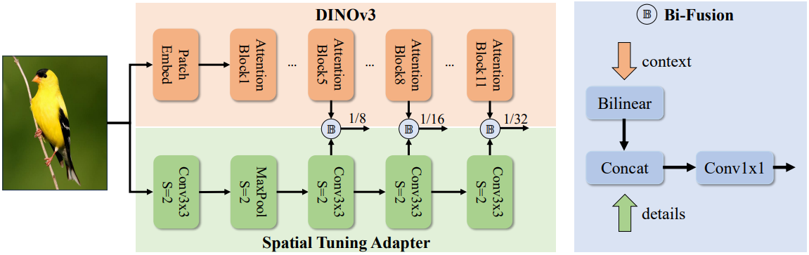
Leveraging DINOv3 with the Spatial Tuning Adapter (STA)
The main challenge in using Vision Transformer (ViT) based models like DINOv3 for object detection is that they naturally produce single-scale feature maps. However, detecting objects of various sizes requires multi-scale features. DEIMv2 solves this elegantly with the Spatial Tuning Adapter (STA).
- Parallel Processing: The STA is a lightweight convolutional neural network (CNN) that runs in parallel with the main DINOv3 backbone. While DINOv3 excels at capturing rich, global semantic context (understanding what is in the image), the STA focuses on extracting fine-grained, multi-scale spatial details (understanding where things are with precision).
- Feature Fusion: The STA takes features from different layers of the DINOv3 backbone, resizes them, and fuses them with its own detailed feature maps using a Bi-Fusion operator. This process effectively converts DINOv3’s powerful but single-scale output into the rich, multi-scale features needed for detecting both large and small objects.
- Parameter Efficiency: This parallel design is highly efficient. It allows DEIMv2 to harness the full power of a pre-trained foundation model without needing to heavily modify or retrain it, saving both parameters and computational cost.
Tailored Backbones for Every Scale
DEIMv2 employs two distinct backbone strategies to cover the full performance spectrum:
- ViT-Based Variants (S, M, L, X): The larger models use official DINOv3-pretrained ViT backbones. This provides them with incredibly strong semantic understanding, leading to top-tier accuracy.
- HGNetv2-Based Variants (Nano, Pico, Femto, Atto): For the ultra-lightweight models, DEIMv2 builds upon the highly efficient HGNetv2 architecture. The authors progressively prune the network’s depth and width to create extremely compact models that can run on low-power devices.
This dual-backbone approach is the secret to DEIMv2’s exceptional scalability.
How Does Its Performance Compare to Other Models?
DEIMv2 sets new state-of-the-art benchmarks across the board, outperforming popular models like the YOLO series, D-FINE, and even its predecessor, DEIM.
Quantitative Results
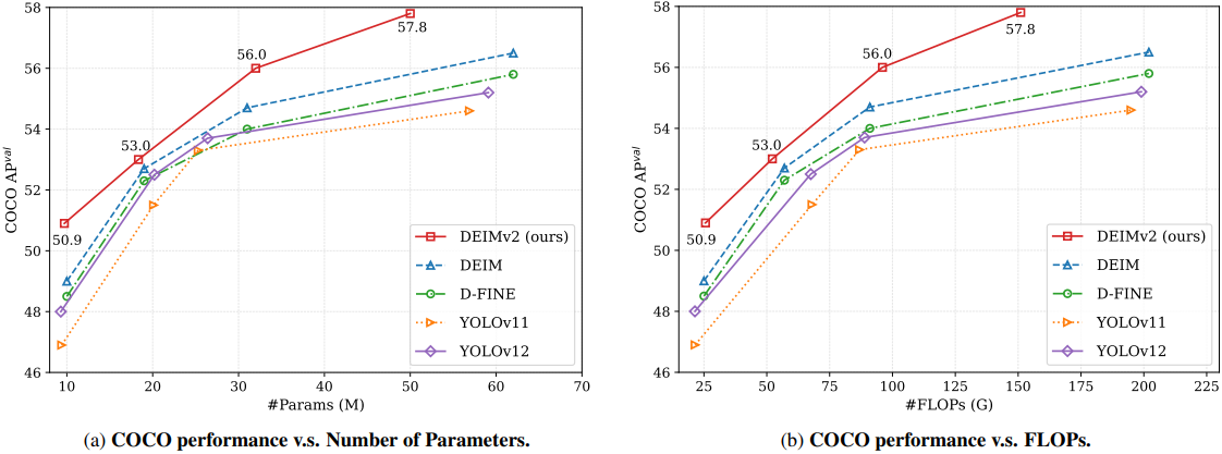
The results on the COCO benchmark speak for themselves:
- The largest model, DEIMv2-X, achieves a remarkable 57.8 AP with only 50.3M parameters. This surpasses previous best models, which required over 60M parameters to reach lower accuracy levels.
- DEIMv2-S becomes the first model with fewer than 10 million parameters to exceed 50 AP on COCO, a significant milestone for compact detectors. It achieves 50.9 AP with just 9.7M parameters.
- The ultra-lightweight DEIMv2-Pico achieves 38.5 AP with a mere 1.5M parameters. This matches the performance of YOLOv10-Nano while using approximately 50% fewer parameters.
Qualitative Results

An interesting finding from the paper is that the performance gains from DINOv3 are most significant for medium and large objects. This is because DINOv3’s strength lies in capturing global context and strong semantics. While small object detection remains a challenge, the overall improvement solidifies DEIMv2’s position as a top-performing real-time detector.
Which Datasets Has DEIMv2 Been Evaluated On?
DEIMv2 was rigorously trained and evaluated on the Microsoft COCO (Common Objects in Context) dataset, which is the industry standard for benchmarking object detection models. The comprehensive evaluation on its val2017 split demonstrates the model’s robustness and generalizability across a wide variety of object classes and scenes.
What Real-Life Use Cases Can We Use DEIMv2 For?
The exceptional scalability of the DEIMv2 framework opens up a vast range of practical applications.
- Autonomous Driving and Robotics: The high-accuracy X and L models can be used for critical tasks like vehicle, pedestrian, and obstacle detection, where precision is non-negotiable.
- High-Throughput Industrial Inspection: In manufacturing, these models can power automated quality control systems, identifying defects on production lines at high speed.
- On-Device Mobile Applications: The lightweight Nano, Pico, and Femto models are perfect for mobile apps, enabling features like real-time object recognition, augmented reality filters, and smart camera functionalities without relying on the cloud.
- Smart Surveillance and Retail Analytics: Edge devices equipped with DEIMv2 can perform on-site video analysis for security monitoring or tracking customer behavior in stores, ensuring privacy and low latency.
The unified nature of DEIMv2 means developers can train a model once and then easily scale it down or up to deploy across different hardware platforms, drastically simplifying the development-to-deployment pipeline.
In the next section, we will explore how to run inference using a pre-trained DEIMv2 model to perform real-time object detection on our own images and videos.
Object Detection Inference with DEIMv2
From this section onward, we will cover the practical aspects, which include:
- Setting up the codebase for running inference.
- Writing the code for image and video inference with DEIMv2.
- Running object detection experiments with DEIMv2 and analyzing the results.
The Project Directory Structure
Let’s take a look at the project directory structure.
├── DEIMv2
│   ├── configs
│   │   ├── base
│   │   ├── dataset
│   │   ├── deim_dfine
│   │   ├── deim_rtdetrv2
│   │   ├── deimv2
│   │   └── runtime.yml
│   ├── dinov3
│   │   ├── dinov3
│   │   ├── __pycache__
│   │   ├── CODE_OF_CONDUCT.md
│   │   ├── conda.yaml
│   │   ├── CONTRIBUTING.md
│   │   ├── hubconf.py
│   │   ├── LICENSE.md
│   │   ├── MODEL_CARD.md
│   │   ├── pyproject.toml
│   │   ├── README.md
│   │   ├── requirements-dev.txt
│   │   ├── requirements.txt
│   │   └── setup.py
│   ├── engine
│   │   ├── backbone
│   │   ├── core
│   │   ├── data
│   │   ├── deim
│   │   ├── misc
│   │   ├── optim
│   │   ├── __pycache__
│   │   ├── solver
│   │   └── __init__.py
│   ├── figures
│   │   ├── deimv2_coco_AP_vs_GFLOPs.png
│   │   └── deimv2_coco_AP_vs_Params.png
│   ├── models
│   │   ├── deimv2_dinov3_l_coco.pth
│   │   ...
│   │   └── deimv2_hgnetv2_pico_coco.pth
│   ├── outputs
│   │   ├── deimv2_dinov3_l_coco_image_1.jpg
│   │   ...
│   │   └── deimv2_hgnetv2_pico_coco_video_2.mp4
│   ├── tools
│   │   ├── benchmark
│   │   ├── dataset
│   │   ├── deployment
│   │   ├── inference
│   │   │   ├── onnx_inf.py
│   │   │   ├── openvino_inf.py
│   │   │   ├── requirements.txt
│   │   │   ├── torch_inf_new.py
│   │   │   ├── torch_inf.py
│   │   │   ├── torch_inf_vis.py
│   │   │   └── trt_inf.py
│   │   ├── reference
│   │   └── visualization
│   ├── LICENSE
│   ├── README.md
│   ├── requirements.txt
│   └── train.py
├── input
│   ├── image_1.jpg
│   ├── image_2.jpg
│   ├── video_1.mp4
│   └── video_2.mp4
└── NOTES.md
- We have two top-level directories. The
DEIMv2directory is the official DEIMv2 repository. Theinputdirectory contains the images and videos on which we will run inference. - Additionally, inside the
DEIMv2directory, we have manually created amodelsdirectory where all the model weights are present. - Finally, inside the
tools/inferencedirectory, we have a custom inference script,torch_inf_new.py. This is an adaptation of thetorch_inf.pyinside the same directory that we will cover in the next section.
The input files and custom inference scripts are provided via a zip file in the download section. The article next covers setting up the repository, handling dependencies, and downloading model weights.
Download Code
Setup and Dependencies
You can first download the zip file containing the input directory and the custom inference script.
Clone the official repository:
After extracting it, we need to clone the DEIMv2 repository inside the directory.
git clone https://github.com/Intellindust-AI-Lab/DEIMv2.git
cd DEIMv2
Installing requirements:
Next, open a terminal inside the cloned DEIMv2 directory and install the requirements.
pip install -r tools/inference/requirements.txt
Downloading Models:
We have to download the model weights for inference. Create a models directory inside the DEIMv2 directory and download and store the weights from here.
This covers all the setup we need.
Inference Script for DEIMv2 Object Detection
The repository comes with an inference script (torch_inf.py) inside the tools/inference directory. However, it is a bit limited in terms of visualization and storing the results. So, we adapt it and create a new torch_inf_new.py inside the same directory.

Let’s cover the code briefly here.
Imports and Output Directory
First, we handle the import statements and create an output directory to store results.
import os
import sys
import time

import cv2  # Added for video processing
import numpy as np
import torch
import torch.nn as nn
import torchvision.transforms as T
from PIL import Image, ImageDraw

sys.path.append(os.path.abspath(os.path.join(os.path.dirname(__file__), '../../')))
from engine.core import YAMLConfig
from engine.data.dataset.coco_dataset import mscoco_label2category, mscoco_category2name

np.random.seed(42)

COLORS = np.random.uniform(0, 255, size=(len(mscoco_label2category), 3))

out_dir = 'outputs'
os.makedirs(out_dir, exist_ok=True)
We also define a COLORS list for the bounding boxes of each COCO category.
Helper Function for Annotation
We need a helper function for annotating frames/images with bounding boxes and texts.
def draw(image, labels, boxes, scores, thrh=0.4):
    image = cv2.cvtColor(np.array(image), cv2.COLOR_RGB2BGR)

    scr = scores
    lab = labels[scr > thrh]
    box = boxes[scr > thrh]
    scrs = scr[scr > thrh]

    for j, b in enumerate(box):
        label = mscoco_category2name[mscoco_label2category[lab[j].item()]]
        cv2.rectangle(
            image,
            pt1=(int(b[0]), int(b[1])),
            pt2=(int(b[2]), int(b[3])),
            color=COLORS[lab[j].item()],
            thickness=2,
            lineType=cv2.LINE_AA
        )
        cv2.putText(
            image,
            text=label,
            org=(int(b[0]), int(b[1]-5)),
            fontFace=cv2.FONT_HERSHEY_SIMPLEX,
            color=COLORS[lab[j].item()],
            thickness=2,
            fontScale=0.8,
            lineType=cv2.LINE_AA
        )

    return image
Functions for Processing Images and Video Frames
The same script can handle both images and videos. So, we have two helper functions for forward passing the inputs in the necessary manner.
def process_image(model, device, file_path, size=(640, 640), model_name=None):
    file_path = os.path.normpath(file_path)
    file_name = file_path.split(os.path.sep)[-1]

    im_pil = Image.open(file_path).convert('RGB')
    w, h = im_pil.size
    orig_size = torch.tensor([[w, h]]).to(device)

    transforms = T.Compose([
        T.Resize(size),
        T.ToTensor(),
    ])
    im_data = transforms(im_pil).unsqueeze(0).to(device)

    output = model(im_data, orig_size)
    labels, boxes, scores = output

    image = draw(im_pil, labels, boxes, scores)

    cv2.imwrite(os.path.join(out_dir, model_name+'_'+file_name), image)


def process_video(model, device, file_path, size=(640, 640), model_name=None):
    fps_counter = 0 # To keep total count of fps.

    file_path = os.path.normpath(file_path)
    file_name = file_path.split(os.path.sep)[-1]
    cap = cv2.VideoCapture(file_path)

    # Get video properties
    fps = cap.get(cv2.CAP_PROP_FPS)
    orig_w = int(cap.get(cv2.CAP_PROP_FRAME_WIDTH))
    orig_h = int(cap.get(cv2.CAP_PROP_FRAME_HEIGHT))

    # Define the codec and create VideoWriter object
    fourcc = cv2.VideoWriter_fourcc(*'mp4v')
    out = cv2.VideoWriter(
        os.path.join(out_dir, model_name+'_'+file_name), fourcc, fps, (orig_w, orig_h)
    )

    transforms = T.Compose([
        T.Resize(size),
        T.ToTensor(),
    ])

    frame_count = 0
    print("Processing video frames...")
    while cap.isOpened():
        ret, frame = cap.read()
        if not ret:
            break

        # Convert frame to PIL image
        frame_pil = Image.fromarray(cv2.cvtColor(frame, cv2.COLOR_BGR2RGB))

        w, h = frame_pil.size
        orig_size = torch.tensor([[w, h]]).to(device)

        im_data = transforms(frame_pil).unsqueeze(0).to(device)

        start_time = time.time()
        output = model(im_data, orig_size)
        end_time = time.time()

        print(f"Forward pass time: {end_time - start_time} seconds")
        fps = int(1 / (end_time - start_time))
        print(f"FPS: {fps}")
        fps_counter += fps

        labels, boxes, scores = output

        # Draw detections on the frame
        frame = draw(frame_pil, labels, boxes, scores)

        # Write the frame
        out.write(frame)
        frame_count += 1

        if frame_count % 10 == 0:
            print(f"Processed {frame_count} frames...")

    cap.release()
    out.release()

    avg_fps = fps_counter / frame_count

    print(f"Average FPS: {avg_fps:.1f}")
Along with handling the forward pass, they also create the output file inside the outputs directory. The output file name is a combination of the original file and the model used for inference. This helps differentiate the results easily.
Main Function and Main Block
Finally, the main function and the main code block.
def main(args):
    """Main function"""
    cfg = YAMLConfig(args.config, resume=args.resume)

    if 'HGNetv2' in cfg.yaml_cfg:
        cfg.yaml_cfg['HGNetv2']['pretrained'] = False

    if args.resume:
        checkpoint = torch.load(args.resume, map_location='cpu')
        if 'ema' in checkpoint:
            state = checkpoint['ema']['module']
        else:
            state = checkpoint['model']
    else:
        raise AttributeError('Only support resume to load model.state_dict by now.')

    # Load train mode state and convert to deploy mode
    cfg.model.load_state_dict(state)

    class Model(nn.Module):
        def __init__(self):
            super().__init__()
            self.model = cfg.model.deploy()
            self.postprocessor = cfg.postprocessor.deploy()

        def forward(self, images, orig_target_sizes):
            outputs = self.model(images)
            outputs = self.postprocessor(outputs, orig_target_sizes)
            return outputs

    device = args.device
    model = Model().to(device)
    img_size = cfg.yaml_cfg["eval_spatial_size"]

    # Check if the input file is an image or a video
    file_path = args.input
    model_name = os.path.normpath(args.config).split(os.path.sep)[-1].split('.yml')[0]
    if os.path.splitext(file_path)[-1].lower() in ['.jpg', '.jpeg', '.png', '.bmp']:
        # Process as image
        process_image(model, device, file_path, img_size, model_name)
        print("Image processing complete.")
    else:
        # Process as video
        process_video(model, device, file_path, img_size, model_name)


if __name__ == '__main__':
    import argparse
    parser = argparse.ArgumentParser()
    parser.add_argument('-c', '--config', type=str, required=True)
    parser.add_argument('-r', '--resume', type=str, required=True)
    parser.add_argument('-i', '--input', type=str, required=True)
    parser.add_argument('-d', '--device', type=str, default='cpu')
    args = parser.parse_args()
    main(args)
We can pass the model configuration, the model weights, the input file, and the computation device as command line arguments.
All the image and video inference experiments were run on a system with 10GB RTX 3080, 10th generation i7 CPU, and 32GB RAM.
Image Inference Experiments with DEIMv2
Let’s start with image inference. We will use the largest model DEIMv3 with DINOv3 backbone for this, i.e., deimv2_dinov3_x_coco. The model contains 50.3 million parameters.
python tools/inference/torch_inf_new.py \
-c configs/deimv2/deimv2_dinov3_x_coco.yml \
-r models/deimv2_dinov3_x_coco.pth \
--input ../input/image_1.jpg \
--device cuda:0
We provide the paths to the model configuration file, the weight file, the image, and the computation device as command line arguments.
The following are inference results from two images.

The model is performing pretty well here.
For the outdoor scene on the right, it can detect the dogs that are even partially hidden. It is detecting all the persons and even the handbag of one of the persons.
For the indoor scene on the left, the detections also look good. It is able to detect some of the partially hidden items, like the broccoli. However, it is sometimes confusing between a cup and a wine glass for similar objects.
Video Inference Experiments with DEIMv2
For the video inference, we will conduct two sets of experiments:
- One using the largest deimv2_dinov3_x_coco model.
- The other is comparing the FPS of the HGNetv2 based backbone models on CPU and GPU.
Let’s run the first one using the deimv2_dinov3_x_coco model.
python tools/inference/torch_inf_new.py \
-c configs/deimv2/deimv2_dinov3_x_coco.yml \
-r models/deimv2_dinov3_x_coco.pth \
--input ../input/video_1.mp4 \
--device cuda:0
The command remains similar; we only change the input file path.
Let’s take a look at the results.
Overall, the results are good. For example, it is able to detect the skateboard in most scenes. However, there are some noticeable issues, such as the switching between the backpack and the handbag.
On the RTX 3080 GPU, the model was running at an average of 26 FPS.
Video Experiments with HGNetv2 Backbone DEIMv2 Models
Moving to the next set of experiments.
The HGNetv2 based DEIMv2 models are some of the most ultra-lightweight models for detection. The DEIMv2 HGNetv2 models include:
- Atto with 0.5M parameters
- Femto with 1.0M parameters
- Pico with 1.5M parameters
- Nano with 3.6M parameters
We will carry out experiments with the first three.
It would be interesting to see the results on both GPU and CPU for these models. Let’s run the inference on the GPU first on another video on the Atto model.
python tools/inference/torch_inf_new.py \
-c configs/deimv2/deimv2_hgnetv2_atto_coco.yml \
-r models/deimv2_hgnetv2_atto_coco.pth \
--input ../input/video_2.mp4 \
--device cuda:0
The following is the result.
As this is the smallest model, there is a lot of flickering in the detections. Also, the model is unable to detect the sports ball in most frames. However, we get an average of 77 FPS with this model, which is really good.
Next, we have the Femto model.
python tools/inference/torch_inf_new.py \
-c configs/deimv2/deimv2_hgnetv2_femto_coco.yml \
-r models/deimv2_hgnetv2_femto_coco.pth \
--input ../input/video_2.mp4 \
--device cuda:0
There seems to be less flickering in the person detection in this case. However, interestingly, the average FPS is 74, just a 3 FPS drop compared to the smallest model.
Finally, the Pico model with 1.5M parameters.
python tools/inference/torch_inf_new.py \
-c configs/deimv2/deimv2_hgnetv2_pico_coco.yml \
-r models/deimv2_hgnetv2_pico_coco.pth \
--input ../input/video_2.mp4 \
--device cuda:0
We have the most stable results in this case, with an average of 70 FPS.
Interestingly, all of these small models are extremely performant in terms of speed on the GPU.
FPS Benchmark Between the HGNetv2 Based DEIMv2 Models
For running the inference on CPU, we just need to change the --device cuda:0 to --device cpu. Following is an example command:
python tools/inference/torch_inf_new.py \
-c configs/deimv2/deimv2_hgnetv2_atto_coco.yml \
-r models/deimv2_hgnetv2_atto_coco.pth \
--input ../input/video_2.mp4 \
--device cpu
After running the experiments, we have the following FPS benchmarks on both CPU and GPU for the HGNetv2 Backbone DEIMv2 models.
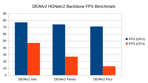
On the 10th generation i7 CPU, the smallest model, Atto runs at 47 FPS, Femto runs at 27 FPS, and Pico runs at 13 FPS. Although the FPS drop from one model to another seems quite significant, we cannot comment much after testing these models on an i7 CPU only. As per the authors, these are meant for edge devices, so more varied benchmarks are necessary. We will try to cover these in future articles.
Summary and Conclusion
In this article, we covered the new DEIMv2 object detection models, which are based on two backbones, DINOv3 and HGNetv2. We started with a discussion of the paper and then moved to inference. We carried out inference on images and videos, and compared the speed for the smallest DEIMv2 models. More benchmarking and custom task training will give better insights that we will cover in future articles.
If you have any questions, thoughts, or suggestions, please leave them in the comment section. I will surely address them.
You can contact me using the Contact section. You can also find me on LinkedIn, and X.
