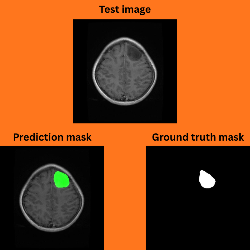
In this article, we are going to use the I-JEPA model for semantic segmentation. We will be using transfer learning to train a pixel classifier head using one of the pretrained backbones from the I-JEPA series of models. Specifically, we will train the model for brain tumor segmentation.
Figure 1. Prediction mask and ground truth mask comparison after training I-JEPA for semantic segmentation task.
This is the fourth part of the I-JEPA series. Previously, we discussed the I-JEPA paper and architecture, image similarity, and image classification using I-JEPA.
This article covers the following regarding semantic segmentation using I-JEPA:
What codebase will we use for training the I-JEPA model for image segmentation?
How do we modify the I-JEPA architecture for segmentation?
Training and inference.
The Semantic Segmentation Dataset for Training I-JEPA
We will use the BRISC 2025 dataset from Kaggle for training a semantic segmentation model using I-JEPA.
The dataset contains tasks for both image classification and semantic segmentation. In one of the previous articles, we trained an image classification model using I-JEPA. In this article, we will make use of the semantic segmentation samples.
We get the following directory structure after downloading and extracting the dataset.
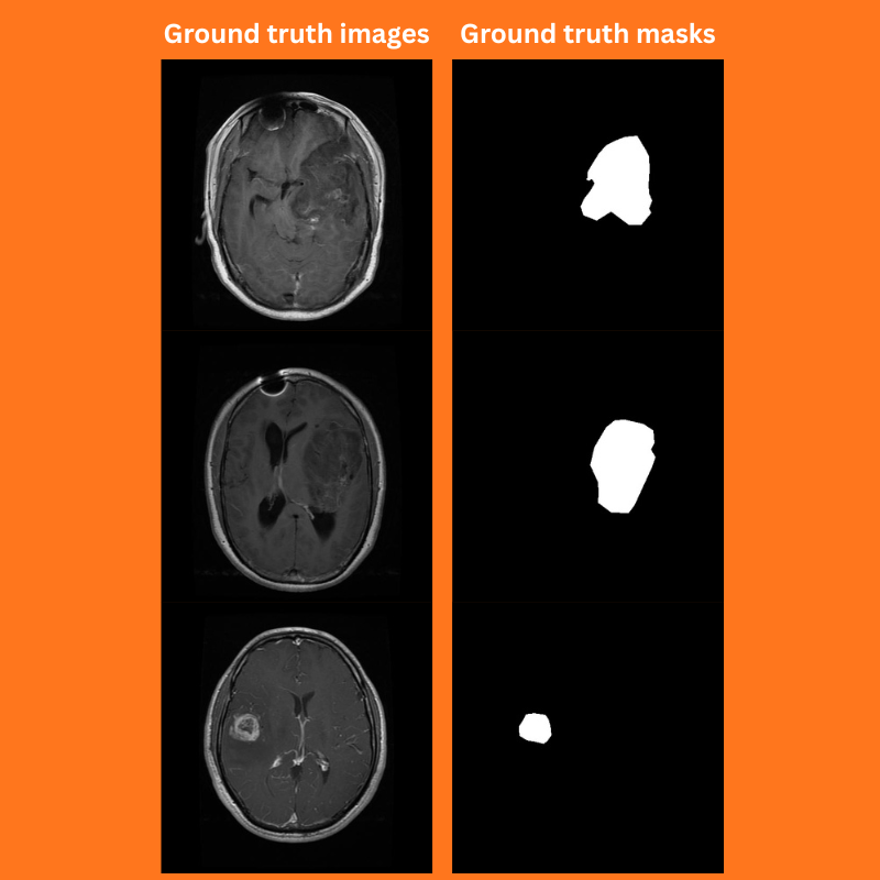
The segmentation_task subdirectory contains the image and masks for the training and validation. The masks are in grayscale format.
Figure 2. Ground truth images and masks from the BRISC 2025 dataset.
There are 3933 training and 869 validation samples.
The I-JEPA Codebase
Currently, I am maintaining a fork of the I-JEPA codebase that supports training and inference for image classification and semantic segmentation.
You need not clone and use the repository. As we are going to make some changes to the codebase for this article, the entire codebase will be available for download.
The img_seg subdirectory inside the src directory contains the code for semantic segmentation dataset preparation, training & evaluation, and utilities.
The input directory contains the BRISC 2025 dataset that we downloaded earlier.
In the parent project directory we have several task specific runnable scripts. Among these, we will focus on the train_segmentation.py, infer_seg_image.py, and create_seg_overlap.py.
If you wish to train the model yourself, please download the BRISC 2025 dataset and arrange it in the above structure. If you want to run inference, then you can download the trained weights from here on Kaggle, and put them in the outputs/img_seg directory.
Download Code
Semantic Segmentation Using I-JEPA
Let’s jump into the necessary parts of the codebase for training I-JEPA for semantic segmentation. As the codebase is quite extensive, we will go through the most important files briefly.
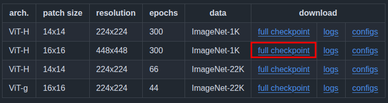
Figure 3. We will use the ViT-H model, pretrained on the ImageNet1K dataset with 16×16 patches and 448×448 image resolution.
The I-JEPA Model for Segmentation
The I-JEPA model is like a large pretrained backbone. You can find more about the I-JEPA model here.
We need a modified architecture for creating a semantic segmentation model out of it. The code for that is present in src/img_seg/model.py. The following block contains the entire code from that file.
import torch
import torch.nn as nn
import math

from collections import OrderedDict
from src.models.vision_transformer import vit_huge
from torchinfo import summary

def load_model(weights):
    model = vit_huge(patch_size=16, img_size=[448])
    print('#'*30, 'Model', '#'*30, )
    print(model)
    print('#'*67)

    if weights is not None:
        ckpt = torch.load(weights, map_location='cpu')
        print(ckpt.keys())
        ckpt_encoder = ckpt['encoder']

        for k, v in ckpt_encoder.items():
            model.state_dict()[k[len('module.'):]].copy_(v)

    model = model.eval()

    return model

class SimpleDecoder(nn.Module):
    def __init__(self, in_channels, nc=1):
        super().__init__()
        self.decode = nn.Sequential(
            nn.Conv2d(in_channels, nc, kernel_size=3)
        )

    def forward(self, x):
        return self.decode(x)

class JepaSegmentation(nn.Module):
    def __init__(self, fine_tune=False, weights=None, num_classes=2):
        super(JepaSegmentation, self).__init__()

        self.backbone_model = load_model(weights=weights)

        self.num_classes = num_classes

        if fine_tune:
            for name, param in self.backbone_model.named_parameters():
                param.requires_grad = True
        else:
            for name, param in self.backbone_model.named_parameters():
                param.requires_grad = False

        self.decode_head = SimpleDecoder(
            in_channels=1280, nc=self.num_classes
        )

        self.model = nn.Sequential(OrderedDict([
            ('backbone', self.backbone_model),
            ('decode_head', self.decode_head)
        ]))

    def forward(self, x):
        # Backbone forward pass
        features = self.model.backbone(x)

        # Reshape patch tokens to (B, EmbeddingDim, patch_h, patch_w)
        B, N, D = features.shape
        tokenH = tokenW = int(math.sqrt(N))

        # Need to correctly resize and permute.
        x = features.view(B, tokenH, tokenW, D)
        x = x.permute(0, 3, 1, 2)  # (B, EmbeddingDim, patch_h, patch_w)

        # Decoder forward pass
        classifier_out = self.model.decode_head(x)
        return classifier_out


if __name__ == '__main__':
    from PIL import Image
    from torchvision import transforms
    import numpy as np

    input_size = 448

    transform = transforms.Compose([
        transforms.Resize(
            input_size,
            interpolation=transforms.InterpolationMode.BICUBIC
        ),
        transforms.CenterCrop(input_size),
        transforms.ToTensor(),
        transforms.Normalize(
            mean=(0.5, 0.5, 0.5),
            std=(0.5, 0.5, 0.5)
        )
    ])

    # Loading the pretrained model without classification head.
    # The following weights path should be relative to the directory
    # from where this module is being executed from.
    weights = 'weights/IN1K-vit.h.16-448px-300e.pth.tar'

    model = JepaSegmentation(fine_tune=False, weights=weights, num_classes=2)
    model.eval()
    print(model)

    random_image = Image.fromarray(np.ones(
        (input_size, input_size, 3), dtype=np.uint8)
    )
    x = transform(random_image).unsqueeze(0)

    with torch.no_grad():
        outputs = model(x)

    print(outputs.shape)

    summary(
        model,
        input_data=x,
        col_names=('input_size', 'output_size', 'num_params'),
        row_settings=['var_names'],
    )
The load_model function loads the pretrained weights, that is, IN1K-vit.h.16-448px-300e.pth.tar present in the weights directory.
We add a simple one layer pixel classifier on top of the backbone, that we define in the SimpleDecoder class. It simply accepts the input channels, from the last layer of the backbone, the number of classes in the dataset, and provides the decoded mask.
The heavy lifting is done in the JepaSegmentation class.
It loads the pretrained weights if we want to fine-tune the model. The forward method first passes the image features via the backbone, which gives us features of shape [batch_size, num_patches, embedding_dim]. Then we reshape and permute them appropriately before passing them over to the pixel classifier head.
The Dataset Preparation
We need some changes to the dataset preparation steps for the BRISC 2025 dataset. Although the masks appear to be binary, the pixel values for the segmentation regions vary between 1 and 255. They can be 240, 245, and so on.
However, we will consider any pixel value above 200 to be a mask region for the tumor. So, in the SegmentationDataset class of src/img_seg/datasets.py, we make the following change when the dataset contains two classes (background and object).
# Make all pixel > 0 as 255.
if len(self.all_classes) == 2:
    im = mask > 200
    mask[im] = 255
    mask[np.logical_not(im)] = 0
Any pixel value that is above 200, make it 255, and the rest as 0.
For the image transforms and augmentation, we use the Albumentations library. The training dataset goes under the following augmentations:
Horizontal flipping
Rotation
Random brightness and contrast
The above augmentations prevent early overfitting and let us train the model longer.
The Dataset Configuration
Each dataset in semantic segmentation can have a different color palette for the masks. Due to this, for correct training, we need to maintain a configuration file. In the codebase, all these configurations are present in the segmentation_configs directory.
For the BRISC 2025 dataset, the configurations are present in the brisc.yaml file and the following are its contents.
The LABEL_COLORS_LIST is used during the dataset preparation. The color values represent the palettes used for different objects. For background, it is black, and for the object, it is white. This should match the values used in the ground truth masks.
The VIS_LABEL_MAP is used for visualization during inference. Instead of white, we use green for visualization.
The Metrics, Training Logic, and Utilities
There are a few other files for which we are skipping the discussion on here. They are the code for evaluation metric, the training & validation loop, and utility & helper functions. However, you can find them in the metrics.py, engine.py, and utils.py in the src/img_seg directory.
We will be using the mean Intersection Over Union as our primary metric to track the model’s progress.
The Runnable Training Script – train_segmentation.py
The train_segmentation.py file contains the logic to start the training process.
It starts with loading the dataset YAML configuration file to get the classes and color maps. Then it creates the data loaders and finally starts the training process.
There are several command line arguments. however, we will only look at those that we need for this training run.
Training the I-JEPA Model for Semantic Segmentation of Brain Tumor
All the training and inference experiments were run on a machine with 10GB RTX 3080 GPU, i7 10th generation CPU, and 32GB RAM.
The following is the command that we can execute from the terminal in the project’s root directory to start the training process.
--train-images and --train-masks: These two accept the path to the directories where training images and masks are present, respectively.
--valid-images and --valid-masks: Similar to the above, these two arguments accept paths to the validation images and masks, respectively.
--config: This argument accepts the path to the dataset’s configuration YAML file.
--lr: The learning rate for training.
--batch: The batch size for data loaders.
--epochs: Number of epochs to train for.
As we are using a high batch size of 48 here, the learning rate is also higher than usual, 0.001. If you use a batch of 4, 8, or 16, please use a smaller learning rate, such as 0.0005 or 0.0001.
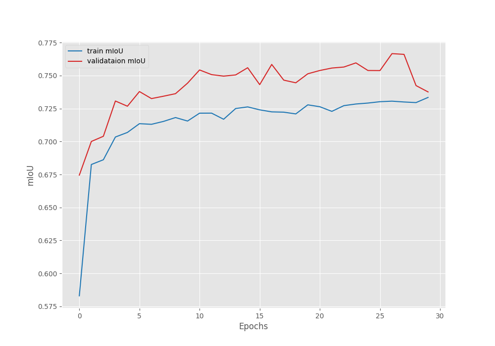
We get the best validation IoU of 76.66% on epoch 27. This is the model we will use for inference.
The following are the accuracy, loss, and IoU graphs.
Figure 4. Accuracy graph after training the I-JEPA model for semantic segmentation.
Figure 5. Loss graph after training the I-JEPA model for semantic segmentation.
Figure 6. Mean IoU graph after training the I-JEPA model for semantic segmentation.
Further training for 10 more epochs with a learning rate scheduler and reducing the learning rate by a factor of 10 from epochs 30 to 40 might help, but is subject to experiment.
Inference on the Test Images
Let’s use the best model to run inference on the test image. The code for inference is present in the infer_seg_image.py file.
We execute the following command with the best model according to IoU, path to the images directory, and path to the dataset configuration file.
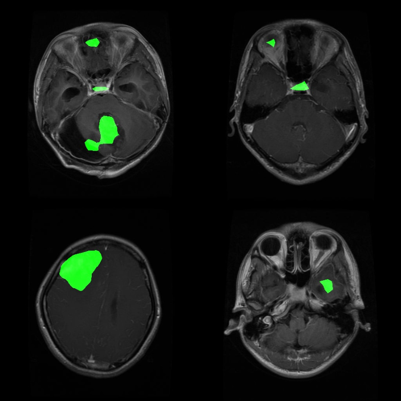
Figure 7. Inference predictions on the test set using the trained I-JEPA model.
Many of us are not medical experts, so we would not be able to determine by sight whether the segmented area is actually a tumor region or not.
To mitigate this, we have another script, create_seg_ovelap.py which creates overlapped images of the inference results on the ground truth test data. Let’s run that and check the results.
python create_seg_ovelap.py
The results will be present in outputs/seg_overlay directory, and you can check all the files on your system.
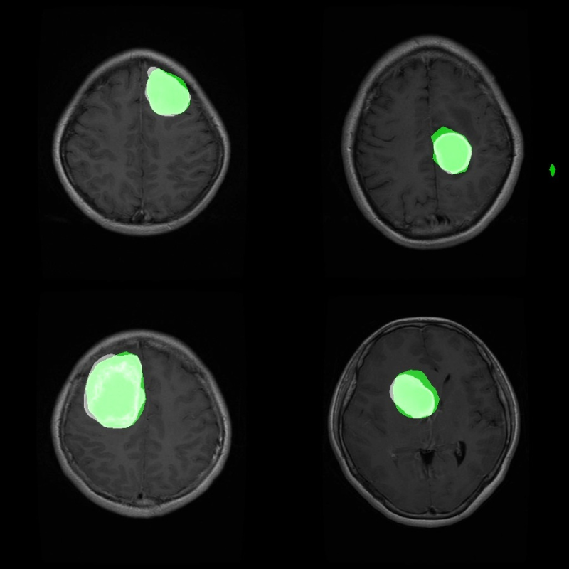
First, let’s analyze some results where the model seems to be performing well. The segmented region in green is the model inference, and white is the ground truth.
Figure 8. A few good segmentation results using the trained I-JEPA model on the BRISC-2025 tumor segmentation dataset.
The above are a few instances where the model seems to be performing somewhat well.
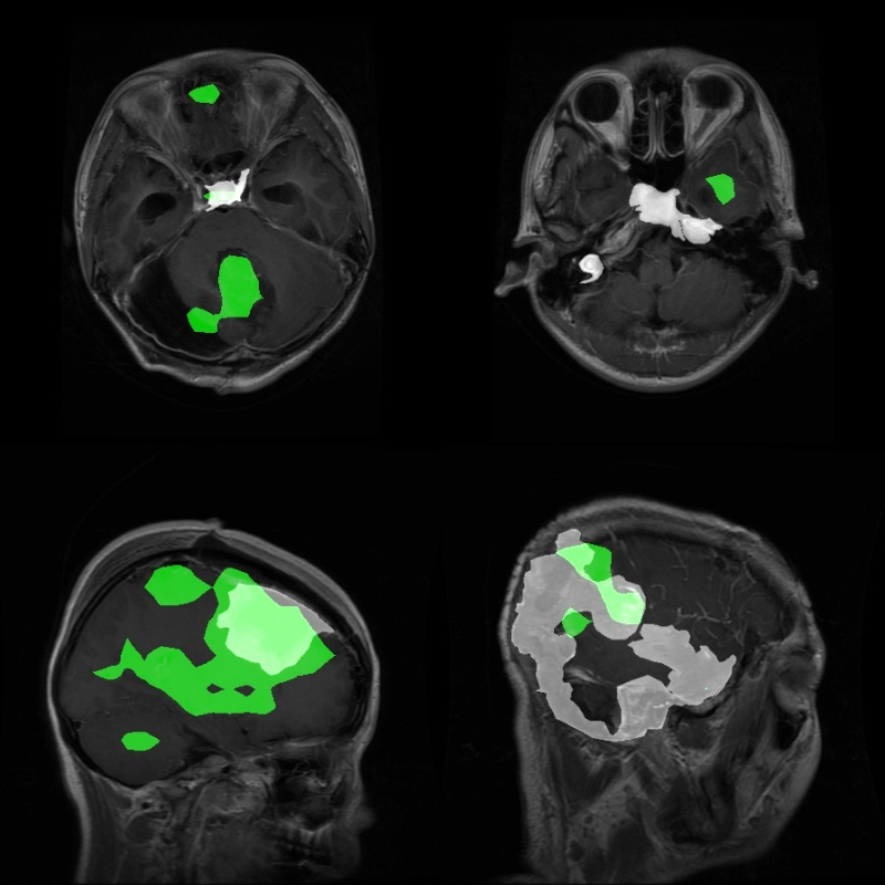
Now, some instances where the model fails.
Figure 9. Inference samples where the trained I-JEPA segmentation model did not perform well.
Clearly, these results are not good.
Takeaways
The above experiment shows some glaring limitations of the model and the approach that we are following. We have used a simple, single-layer pixel classifier for the segmentation head. There is a chance that using a more complex, multi-layer feature aggregator will improve the results.
Furthermore, we can also pretrain such a pixel classifier on COCO segmentation datasets to make it learn complex features. Then we can use it for such complex experiments.
Summary and Conclusion
In this article, we conducted semantic segmentation training experiments using I-JEPA. We trained the model on a tumor segmentation dataset and analyzed the results. Although the entire process gave us a good idea of setting up such a pipeline, the final results were not as good as expected from a model of this scale. We also discussed a few experiments to carry out further, which may improve the results.
If you have any questions, thoughts, or suggestions, please leave them in the comment section. I will surely address them.
You can contact me using the Contact section. You can also find me on LinkedIn, and X.
Liked it? Take a second to support Sovit Ranjan Rath on Patreon!
This website uses cookies so that we can provide you with the best user experience possible. Cookie information is stored in your browser and performs functions such as recognising you when you return to our website and helping our team to understand which sections of the website you find most interesting and useful.
Strictly Necessary Cookies
Strictly Necessary Cookie should be enabled at all times so that we can save your preferences for cookie settings.
If you disable this cookie, we will not be able to save your preferences. This means that every time you visit this website you will need to enable or disable cookies again.