Following the previous article, we have another project combining deep learning and environment. Millions of people all over the world get displaced due to floods. It’s true that by using deep learning + computer vision, we cannot always predict when the next flood will hit. But we can train a semantic segmentation algorithm on images of flood-hit areas. Such a model can help in the analysis and decision-making for future situations. To do our tiny bit, we will train a semantic segmentation model for flood recognition using PyTorch in this article.

If you go through the previous article, you will find that we had ample examples of water body segmentation using the DeepLabV3 model. But the dataset had some apparent issues. Such as wrong ground truth segmentation in some of the images. Also, some of the edges of the images were labeled as water bodies.
In this article, for semantic segmentation for flood recognition, the situation is quite opposite. We have very less but almost perfect data. We will discuss the dataset and its challenges in one of the further sections.
For now, let’s focus on the points that we will cover in the article:
- As usual, we will start by discussing the dataset.
- Next, in the coding section, we will discuss:
- The deep learning semantic segmentation model to use.
- The preparation of the dataset.
- Hyperparameter choices.
- After training the model, we will run inference on the validation images and unseen videos for flood recognition.
- Finally, we will discuss some ways to move this project ahead and what may be possible further.
I hope the premise interests you. Let’s dive into the article now.
The Flood Segmentation Dataset
Flood segmentation may seem similar to the waterbody segmentation from satellite images. We covered the waterbody segmentation project when trying to train the PyTorch DeepLabV3 model on a custom dataset.
But there are more complications when trying to segment flood areas. Let’s explore the dataset first and then discuss it further.
We will use a modified version of the Flood Area Segmentation from Kaggle. It’s a pretty good and clean dataset. But it has some image extension issues and one of the images is corrupted.
I have prepared a modified version of this dataset. This is the Flood Segmentation Dataset Train/Validation Split on Kaggle. We will use this version of the dataset. Here are the changes:
- The dataset now contains a training and validation split.
- There are 257 training images & masks and 32 validation images & masks.
- There are no corrupted images in the dataset now.
After downloading and extracting the dataset, you will find the following structure.
flood-area-segmentation
├── train_images
├── train_masks
├── valid_images
└── valid_masks
All the ground truth images are in RGB format. And all the masks are grayscale images having white pixels (255) for the flood areas and black pixels (0) otherwise. So, it is a binary semantic segmentation dataset. Here are a few images.

Why Is Semantic Segmentation for Flood Recognition Difficult?
Let’s talk about why flood segmentation is difficult in terms of this dataset.
First of all, this dataset contains only 257 training images and masks. Surely, this is not enough to train a state-of-the-art semantic segmentation model. We will need ample augmentation techniques just to keep the loss reducing.
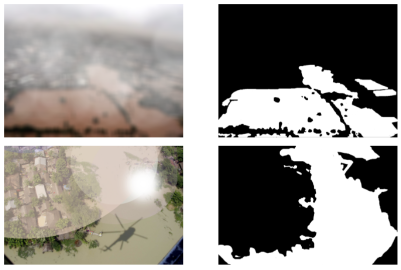
Secondly, there will be many small background pixels in between the flood areas. These can range from houses to agricultural fields, and even partially submerged vehicles.
Here are a few examples of the same.

The model will have to learn these background classes properly and not segment them. For smaller models, this can be particularly challenging.
Keeping the above issues in mind, we will try to train the best model that we can.
PyTorch and Other Dependencies
The code for this project uses TORCH 1.12.0 and TORCHVISION 0.13.0. You can use newer versions as well.
Also, Albumentations is one of the requirements for image and mask augmentations.
Please be sure to install the above two libraries.
Directory Structure for Semantic Segmentation for Flood Recognition
We will follow this directory structure for the project.
.
├── input
│   ├── flood-area-segmentation
│   │   ├── train_images
│   │   ├── train_masks
│   │   ├── valid_images
│   │   └── valid_masks
│   └── inference_data
│       └── video_1.mp4
├── outputs
│   ├── inference_results
│   │   ├── 1005.jpg
│   │   ...
│   │   └── 38.jpg
│   ├── inference_results_video
│   │   └── video_1.mp4
│   ├── valid_preds
│   │   ├── e0_b7.jpg
│   │   ...
│   │   └── e9_b7.jpg
│   ├── accuracy.png
│   ├── best_model.pth
│   ├── loss.png
│   └── model.pth
└── src
    ├── config.py
    ├── datasets.py
    ├── engine.py
    ├── inference_image.py
    ├── inference_video.py
    ├── metrics.py
    ├── model.py
    ├── train.py
    └── utils.py
- The
inputdirectory contains theflood-area-segmentationdataset and theinference_dataalso. - In the
outputsdirectory, we have all the training and inference related outputs. This includes the model weight files, the image results after inference, and the segmentation outputs from the validation loop as well. - The
srcdirectory contains all the Python source code files. As there are 9 Python files, we will not be able to go through each of them in detail. But we will explore the important parts of the code in the next sections.
You will find all the source code files when downloading the zip files that come with this article. In case, you only want to run inference, please find the trained weight files here.
Semantic Segmentation for Flood Recognition using PyTorch and DeepLabV3 ResNet50
From now on, we will discuss the technical aspects of the project. Before starting the training, we will cover these topics:
- Configuration file.
- The deep learning model to use for semantic segmentation for flood recognition.
- The dataset preparation strategy.
- Data augmentations for the training set.
- Training hyperparameters and arguments. These include the optimizer, learning rate, and choice of batch size according to the availability of VRAM. We will also discuss the implications of training image size.
Download Code
The Configuration File
There are a few configurations we will use throughout the project in the rest of the Python files. Instead of re-writing these configurations repeatedly, we will just have a config.py file and store these.
ALL_CLASSES = ['background', 'flood']

LABEL_COLORS_LIST = [
    (0, 0, 0), # Background.
    (255, 255, 255), # Flood.
]

VIS_LABEL_MAP = [
    (0, 0, 0), # Background.
    (255, 0, 0), # Flood.
]
The ALL_CLASSES list contains the names of classes in the dataset.
The LABEL_COLORS_LIST contains tuples of RGB colors as per the dataset. In the dataset, background classes have black colors and the flooded areas have white colors.
Finally, VIS_LABEL_MAP contains the RGB color tuples that we will use for visualization. For clarity, we will use the red color to segment out the flooded regions during inference.
The DeepLabV3 ResNet50 Model for Semantic Segmentation for Flood Recognition
We will use the good, old, reliable DeepLabV3 with ResNet50 backbone for semantic segmentation in this project.
Preparing the model for custom model training is quite easy. In fact, we just the following lines of code to prepare the model for custom semantic segmentation training.
import torch.nn as nn

from torchvision.models.segmentation import deeplabv3_resnet50

def prepare_model(num_classes=2):
    model = deeplabv3_resnet50(weights='DEFAULT')
    model.classifier[4] = nn.Conv2d(256, num_classes, 1)
    model.aux_classifier[4] = nn.Conv2d(256, num_classes, 1)
    return model
To get better performance, we will use pretrained weights. Also, we need to modify the classifier and aux_classifier head according to the number of classes in our dataset. There are two classes in the dataset, one for background and one for flooded areas.
The main reason for choosing DeepLabV3 with ResNet is the speed and performance. In PyTorch we have two other options as well for DeepLabV3:
- With ResNet101 backbone. While it performs well, it requires more memory to train and is also slower during inference.
- And the DeepLabV3 with MobileNet backbone. It is fast but does not perform as well.
For this reason, we choose the best of both worlds with DeepLabV3 ResNet50.
The Dataset Preparation
While we will not go through the entire code for dataset preparation, there are a few important things to take notice of here.
One of them is the data augmentation strategy.
Remember that we have only 257 images and masks for training. This is not enough to train a good model. But data augmentation can help us with this. We will use the Albumentations library to easily apply the augmentations to the images and masks.
We will apply the following augmentations to the training images and masks for the flood segmentation dataset.
- HorizontalFlip
- RandomBrightnessContrast
- RandomSunFlare
- RandomFog
- ImageCompression
Apart from horizontal flipping (applied with 0.5 probability), we will apply all other augmentations with 0.2 probability.
This is what the images will look like after applying these augmentations randomly.
As you can see, only spatial augmentations (flipping) are applied to the masks. Other pixel-level manipulations which affect the color, hue, or saturation are not applied to the masks. This is pretty easy to achieve using Albumentations. Please check the dataset.py file to get more details.
Also, as per the TORCHVISION segmentation models guidelines, we will be using the ImageNet normalizations.
Other than that, we will be handling the image and batch size from the training script’s command line arguments.
Utility Scripts, Metrics, and Training & Validation Code
The utils.py file contains a lot of helper functions and utility classes. These include the class to save the best model, functions to save the accuracy & loss plots, and also functions to overlay segmentation maps on top of images.
The metrics.py contains the pix_acc function. This returns the total number of labeled pixels and the correctly classified pixels. We will use these to calculate the pixel accuracy in the engine.py file.
As such, the engine.py contains the training and validation functions that we will call on each epoch.
If you wish, you may go over the code in these files before we move over to the training section.
Training DeepLabV3 on the Flood Segmentation Dataset
Finally, we are at the point where we can train the DeepLabV3 ResNet50 model on the flood segmentation dataset.
Note: All training and inference experiments were carried on a machine with 10GB RTX 3080 GPU, 10th generation i7 CPU, and 32 GB RAM.
The train.py is the driver script that we will use to kick off the training.
Before we start the training, let’s go over the argument parsers that the training script supports.
--epochs: The number of epochs that we want to train the model.--lr: The learning rate for the optimizer. It is 0.0001 by default.--batch: Batch size for the data loader.--imgsz: The image size we want to train the model with. Semantic segmentation models often need higher resolution images to achieve good results. We will train the model on 512×512 images which is the default value as well.--scheduler: This is a boolean flag indicating whether we want to use the learning rate scheduler or not. If we pass this flag then the learning rate will be reduced by a factor of 10 after 25 epochs.
If you face OOM (Out Of Memory) error while training, please consider reducing the image size or the batch size.
We can start the training by executing the following command in the terminal with src as the current working directory.
python train.py --epochs 50 --batch 4 --lr 0.0001 --scheduler
We are training the model for 50 epochs, with a batch size of 4, starting learning rate of 0.0001, and also applying the learning rate scheduler.
Here are the truncated outputs from the terminal.
python train.py --epochs 50 --batch 4 --lr 0.0001 --scheduler
Namespace(epochs=50, lr=0.0001, batch=4, scheduler=True)
41,994,308 total parameters.
41,994,308 training parameters.
Adjusting learning rate of group 0 to 1.0000e-04.
EPOCH: 1
Training
Loss: 0.4229 | PixAcc: 83.23: 100%|████████████████████| 64/64 [00:50<00:00,  1.26it/s]
Validating
Loss: 0.3060 | PixAcc: 89.33: 100%|████████████████████| 8/8 [00:02<00:00,  3.57it/s]

Best validation loss: 0.38311174884438515

Saving best model for epoch: 1

Train Epoch Loss: 0.5018, Train Epoch PixAcc: 64.9515
Valid Epoch Loss: 0.3831, Valid Epoch PixAcc: 86.8635
Adjusting learning rate of group 0 to 1.0000e-04.
--------------------------------------------------
EPOCH: 2
Training
Loss: 0.3776 | PixAcc: 81.60: 100%|████████████████████| 64/64 [00:49<00:00,  1.30it/s]
Validating
Loss: 0.4301 | PixAcc: 91.83: 100%|████████████████████| 8/8 [00:02<00:00,  3.84it/s]
Train Epoch Loss: 0.3887, Train Epoch PixAcc: 72.3201
Valid Epoch Loss: 0.4537, Valid Epoch PixAcc: 94.0050
Adjusting learning rate of group 0 to 1.0000e-04.
--------------------------------------------------
EPOCH: 3
Training
Loss: 0.4062 | PixAcc: 68.83: 100%|████████████████████| 64/64 [00:49<00:00,  1.29it/s]
Validating
Loss: 0.2974 | PixAcc: 93.10: 100%|████████████████████| 8/8 [00:02<00:00,  3.86it/s]
Train Epoch Loss: 0.3698, Train Epoch PixAcc: 75.0250
Valid Epoch Loss: 0.4060, Valid Epoch PixAcc: 94.7763
Adjusting learning rate of group 0 to 1.0000e-04.
--------------------------------------------------
.
.
.
EPOCH: 50
Training
Loss: 0.1831 | PixAcc: 80.59: 100%|████████████████████| 128/128 [00:39<00:00,  3.26it/s]
Validating
Loss: 0.1339 | PixAcc: 98.66: 100%|████████████████████| 16/16 [00:02<00:00,  7.16it/s]
Train Epoch Loss: 0.1459, Train Epoch PixAcc: 91.4595
Valid Epoch Loss: 0.2437, Valid Epoch PixAcc: 88.4480
Adjusting learning rate of group 0 to 1.0000e-06.
--------------------------------------------------
TRAINING COMPLETE
Analyzing the DeepLabV3 Flood Segmentation Results
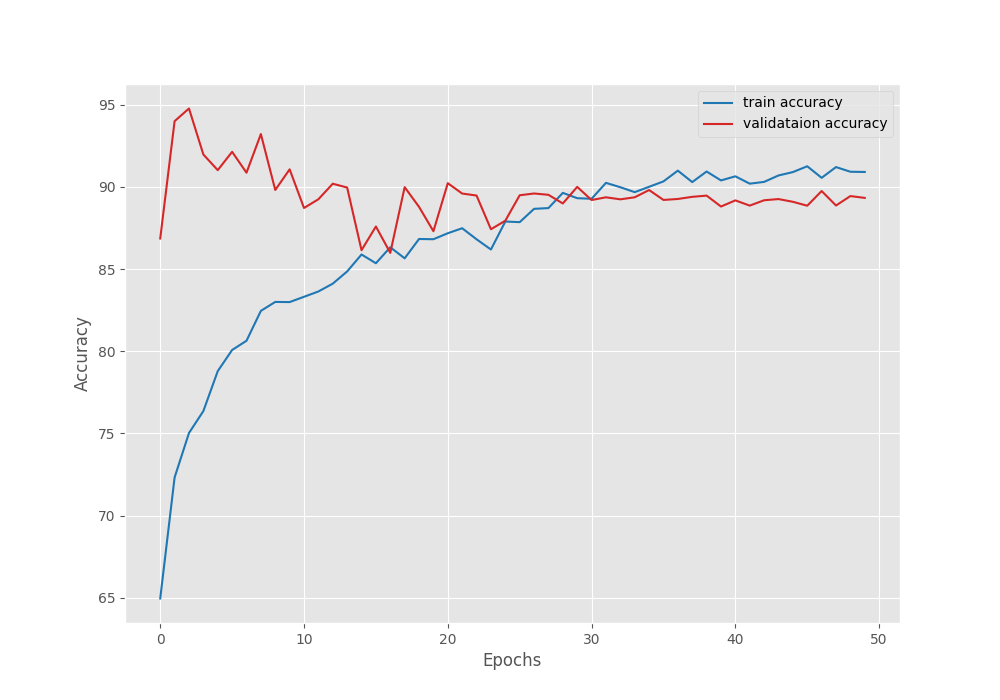
Interestingly, we have the least validation loss of 0.222 on epoch 33 while the highest pixel accuracy is on epoch 3. This is a bit of an odd situation as the best model is saved based on the least loss. Let’s take a look at the accuracy and loss plots.

We can see a lot of fluctuations in the initial epochs and throughout the training till the learning rate drops. This means that we needed the learning rate scheduler. Perhaps we can train with an even lower initial learning rate to mitigate this unstable training.
Anyways, we have a trained model with us for now. Let’s run some inference experiments on images and videos.
Flood Segmentation Inference on Images
For image inference, we will choose the same validation images from the dataset.
To run the inference on images, we will use the inference_image.py script.
python inference_image.py --input ../input/flood-area-segmentation/valid_images/
We use the --input flag to provide the path to the validation images directory.
You can find the results inside outputs/inference_results directory.
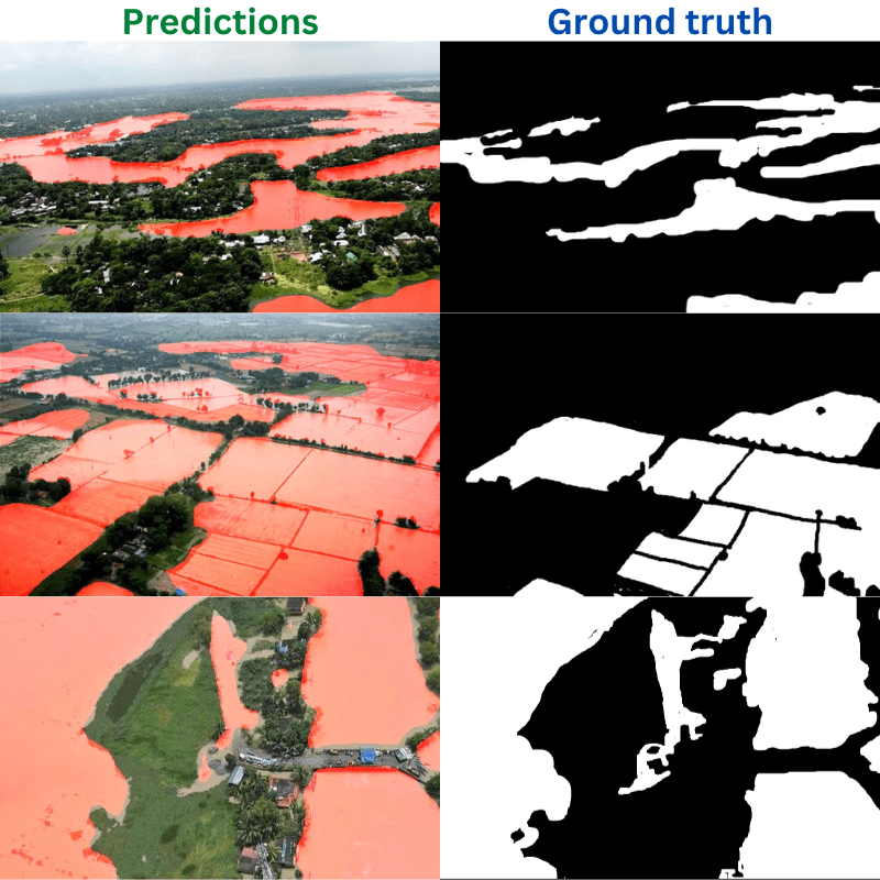
Here are some of the outputs. The first column shows the predictions by the model, and the right column shows the ground truth masks.
While may not be perfect, the results are pretty good. The model still finds it difficult to differentiate between thin lines of land and the flooded area. But that is something that we can rectify with more training data and better training techniques.
Flood Segmentation Inference on Videos
The inference_video.py script contains the code to run inference on videos. We can use it by proving the path to a video file.
python inference_video.py --input ../input/inference_data/video.mp4
On an RTX 3080 GPU, we get an average of 21 FPS. This is not too great as you may consider. We are not resizing the frames before feeding them to the model. Resizing them to 512×512 resolution will increase the FPS a bit.
The following is the output that we get.
The results look pretty good actually. Surely, the model is still segmenting very small patches of land as water. But the results are really good considering we had only 257 training images.
Further Improvements
This project has a lot of potential if we can scale the training data and the training pipeline. Such a deep learning model can be attached to a drone to segment out the flooded areas in a region. This will help make proper plans to restructure a particular region so that such flood situations do not occur in the future.
Summary and Conclusion
In this article, we covered binary semantic segmentation for flood area recognition. Starting from the dataset discussion till the training results, we covered each part. While doing the project, we also got the idea of how we can scale the project to a real-life solution if we can deploy such a model onto a drone. I hope that this article was worth the time.
If you have any doubts, thoughts, or suggestions, please leave them in the comment section. I will surely address them.
You can contact me using the Contact section. You can also find me on LinkedIn, and X.


This is very useful but I need your help how we can run this project so we can see the output can please tell me the mac step how we can run
Hello Hemish. All the directory structure and commands are given in the article. You can follow them. Can you please let me know if you are facing some specific issues.
I’m unable to download the code
Hi. Apologies for the issue. I have sent the code link via email. Please check.