

In the last two articles, we covered image classification and semantic segmentation using DINOv3. This article covers another fundamental downstream task in computer vision, object detection with DINOv3. The object detection task will really test the limits of DINOv3 backbones, as it is one of the most difficult tasks in computer vision when the datasets are small in size.
Here, instead of using one of the ViT backbones as we did in the previous articles, we will use the DINOv3 ConvNeXt Tiny backbone. Furthermore, the training pipeline and the results might not be the best. This article will serve as a starting point for future articles and projects, and readers who might want to take this further.
What will we cover in object detection with DINOv3?
- The Pascal VOC object detection dataset.
- Exploring the DINOv3 Stack codebase for object detection.
- Setting up the project directory and dependencies.
- Discussing the important code snippets – such as modifying the DINOv3 backbone for detection, the dataset creation, and augmentations.
- Training and inference.
The Pascal VOC Object Detection Dataset
The Pascal VOC object detection dataset is perhaps one of the most famous in the history of computer vision. It is repeatedly benchmarked in papers. Given its moderate size, with ~16,500 training and ~5,000 validation samples, it is suitable for experimental training.
To follow along, you can download the dataset from Kaggle. The annotations are present in the XML file format.
We see the following directory structure after downloading and extracting it.
├── voc_07_12
│   └── voc_xml_dataset
│       ├── train
│       │   ├── images  [16551 entries exceeds filelimit, not opening dir]
│       │   └── labels  [16551 entries exceeds filelimit, not opening dir]
│       ├── valid
│       │   ├── images  [4952 entries exceeds filelimit, not opening dir]
│       │   └── labels  [4952 entries exceeds filelimit, not opening dir]
│       └── README.txt
└── readme.txt
Here are some samples from the training dataset along with their ground truth annotations.

The samples are diverse, and that’s what makes the dataset a bit challenging as well. We have just 16500 samples to make the model learn the features in various scenarios.
The DINOv3 Stack Codebase
Following the approach from our previous article, we will continue to use the dinov3_stack GitHub project.
At the time of writing this, I had recently pushed a detection branch containing the initial codebase for object detection using DINOv3. This was eventually merged with the main branch and changes are bound to happen in the near future.
It is still a work in progress, so a lot of the parameters are hardcoded at the moment. Still, it is a fully working codebase, and we will discuss all the necessary parts in their respective subsections.
The Project Directory Structure
Let’s take a look at the project directory structure.
├── classification_configs
│   └── leaf_disease.yaml
├── dinov3
│   ├── dinov3
│   │   ├── checkpointer
│   │   ├── configs
│   │   ├── data
│   │   ...
│   │   └── __init__.py
│   ├── __pycache__
│   │   └── hubconf.cpython-312.pyc
│   ...
│   ├── requirements-dev.txt
│   ├── requirements.txt
│   └── setup.py
├── input
│   ├── voc_07_12
│   │   └── voc_xml_dataset
│   └── readme.txt
├── outputs
│   └── img_det
│       ├── best_model.pth
│       ├── last_model.pth
│       ├── map.png
│       └── train_loss.png
├── segmentation_configs
│   ├── person.yaml
│   └── voc.yaml
├── src
│   ├── detection
│   │   ├── __pycache__
│   │   ├── analyze_dataset.py
│   │   ├── config.py
│   │   ├── custom_utils.py
│   │   ├── datasets.py
│   │   ├── eval.py
│   │   └── model.py
│   ├── img_cls
│   │   ├── datasets.py
│   │   ├── __init__.py
│   │   ├── model.py
│   │   └── utils.py
│   ├── img_seg
│   │   ├── datasets.py
│   │   ├── engine.py
│   │   ├── __init__.py
│   │   ├── metrics.py
│   │   ├── model.py
│   │   └── utils.py
│   └── utils
│       ├── __pycache__
│       └── common.py
├── weights
│   └── dinov3_convnext_tiny_pretrain_lvd1689m-21b726bb.pth
├── infer_classifier.py
├── infer_det_image.py
├── infer_det_video.py
├── infer_seg_image.py
├── infer_seg_video.py
├── License
├── NOTES.md
├── Outputs.md
├── README.md
├── requirements.txt
├── train_classifier.py
├── train_detection.py
└── train_segmentation.py
- Inside the parent project directory, we have the
train_detection.py,infer_det_image.py, andinfer_det_video.py. These are the executable scripts for object training and inference. - The
src/detectionfolder contains all the utility and engine scripts for object detection. - The
outputsdirectory will contain all the training and inference results. - We have also cloned the
dinov3repository, which is necessary to load the pretrained models.
All the source code and trained weights are available via the download section. The remaining part of the setup is covered in the following section.
Download Code
Dependencies and Setup
Cloning the DINOv3 repository
First, we need to clone the DINOv3 repository, which is essential for loading the pretrained weights. You can clone it inside the project directory.
git clone https://github.com/facebookresearch/dinov3.git
Creating a weights directory
Second, we need to create a weights directory and keep the DINOv3 ConvNeXt tiny weights inside that.
mkdir weights
You can download the pretrained weights by filling out the form available via clicking one of the links on the official repository model table.
You should receive an email with the link to the weights. In this article, we are using dinov3_convnext_tiny_pretrain_lvd1689m-21b726bb.pth.
Creating a .env file
Third, we need a .env file in the project directory mentioning the cloned dinov3 and the weights directory path.
# Should be absolute path to DINOv3 cloned repository.
DINOv3_REPO="dinov3"

# Should be absolute path to DINOv3 weights.
DINOv3_WEIGHTS="weights"
Installing the rest of the dependencies
Finally, install the rest of the requirements.
pip install -r requirements.txt
This ends the setup that we need to run DINOv3 for object detection.
Using DINOv3 for Object Detection
Let’s jump into the code. We will discuss the important parts of the code that are necessary to understand the approach.
Modifying DINOv3 Backbone for Object Detection
The very first step is modifying the DINOv3 backbone for object detection.
For detection, we will use the SSD (Single Shot Detection) head from Torchvision, rather than defining a custom head as we did in the case of DINOv3 semantic segmentation.
The code for this is present in the src/detection.model.py file. The following code block contains the import statements and the entire process to create the model.
import torch
import torch.nn as nn
import os

from torchvision.models.detection.ssd import (
    SSD,
    DefaultBoxGenerator,
    SSDHead
)

def load_model(weights: str=None, model_name: str=None, repo_dir: str=None):
    if weights is not None:
        print('Loading pretrained backbone weights from: ', weights)
        model = torch.hub.load(
            repo_dir,
            model_name,
            source='local',
            weights=weights
        )
    else:
        print('No pretrained weights path given. Loading with random weights.')
        model = torch.hub.load(
            repo_dir,
            model_name,
            source='local'
        )

    return model

class Dinov3Backbone(nn.Module):
    def __init__(self,
        weights: str=None,
        model_name: str=None,
        repo_dir: str=None,
        fine_tune: bool=False
    ):
        super(Dinov3Backbone, self).__init__()

        self.model_name = model_name

        self.backbone_model = load_model(
            weights=weights, model_name=model_name, repo_dir=repo_dir
        )

        if fine_tune:
            for name, param in self.backbone_model.named_parameters():
                param.requires_grad = True
        else:
            for name, param in self.backbone_model.named_parameters():
                param.requires_grad = False

    def forward(self, x):
        out = self.backbone_model.get_intermediate_layers(
            x,
            n=1,
            reshape=True,
            return_class_token=False,
            norm=True
        )[0]

        return out

def dinov3_detection(
    fine_tune: bool=False,
    num_classes: int=2,
    weights: str=None,
    model_name: str=None,
    repo_dir: str=None,
    resolution: list=[640, 640],
    nms: float=0.45,
    feature_extractor: str='last' # OR 'multi'
):
    backbone = Dinov3Backbone(
        weights=weights,
        model_name=model_name,
        repo_dir=repo_dir,
        fine_tune=fine_tune
    )

    out_channels = [backbone.backbone_model.norm.normalized_shape[0]] * 6
    anchor_generator = DefaultBoxGenerator(
        [[2], [2, 3], [2, 3], [2, 3], [2], [2]],
    )
    num_anchors = anchor_generator.num_anchors_per_location()

    head = SSDHead(out_channels, num_anchors, num_classes=num_classes)

    model = SSD(
        backbone=backbone,
        num_classes=num_classes,
        anchor_generator=anchor_generator,
        size=resolution,
        head=head,
        nms_thresh=nms
    )

    return model
As of writing this, the codebase supports all the ViT and ConvNeXt backbones. However, we will go with the ConvNeXt tiny model as it is the fastest to train and gives reasonable initial results.
The load_model function:
The load_model function accepts the weight file path, the model name (e.g. dinov3_convnext_tiny), and the DINOv3 repository path. It loads the backbone and returns the instance.
The Dinov3Backbone class:
We need a little bit of control over the forward pass of the backbone before we can feed it to the detection head. So, we create a class (subclassed by nn.Module). As we are not using multi-level feature maps, we return the first element from the forward pass output (lines 53-59).
The dinov3_detection function:
This function aggregates everything to create the detection model. At the moment, the codebase supports SSD head only. The RetinaNet head will be added in the near future.
We initialize the backbone and define the output channel dimensions (line 80). This process is dynamic and will handle any backbone.
Then we define the anchor generator and finally the Single Shot Detection head with DINOv3 backbone.
If you wish to learn more, you can visit this article for custom backbones using SSD head.
The file also contains a main block that does sanity checking by creating an instance of the model and doing a forward pass. We can run it with the following command:
python -m src.detection.model
We get the following output:
==================================================================================================================================
Layer (type (var_name))                                 Input Shape               Output Shape              Param #
==================================================================================================================================
SSD (SSD)                                               [1, 3, 640, 640]          [200, 4]                  --
├─GeneralizedRCNNTransform (transform)                  [1, 3, 640, 640]          [1, 3, 640, 640]          --
├─Dinov3Backbone (backbone)                             [1, 3, 640, 640]          [1, 768, 20, 20]          --
│    └─ConvNeXt (backbone_model)                        --                        --                        --
│    │    └─ModuleList (downsample_layers)              --                        --                        (recursive)
│    │    └─ModuleList (stages)                         --                        --                        (recursive)
│    │    └─ModuleList (downsample_layers)              --                        --                        (recursive)
│    │    └─ModuleList (stages)                         --                        --                        (recursive)
│    │    └─ModuleList (downsample_layers)              --                        --                        (recursive)
│    │    └─ModuleList (stages)                         --                        --                        (recursive)
│    │    └─ModuleList (downsample_layers)              --                        --                        (recursive)
│    │    └─ModuleList (stages)                         --                        --                        (recursive)
│    │    └─ModuleList (norms)                          --                        --                        (1,536)
├─SSDHead (head)                                        [1, 768, 20, 20]          [1, 1600, 21]             --
│    └─SSDRegressionHead (regression_head)              [1, 768, 20, 20]          [1, 1600, 4]              --
│    │    └─ModuleList (module_list)                    --                        --                        829,560
│    └─SSDClassificationHead (classification_head)      [1, 768, 20, 20]          [1, 1600, 21]             --
│    │    └─ModuleList (module_list)                    --                        --                        4,355,190
├─DefaultBoxGenerator (anchor_generator)                [1, 3, 640, 640]          [1600, 4]                 --
==================================================================================================================================
Total params: 33,004,878
Trainable params: 5,184,750
Non-trainable params: 27,820,128
Total mult-adds (Units.GIGABYTES): 2.72
==================================================================================================================================
Input size (MB): 4.92
Forward/backward pass size (MB): 1074.30
Params size (MB): 114.02
Estimated Total Size (MB): 1193.23
==================================================================================================================================
For 21 classes of the VOC detection dataset, the model has approximately 33 million parameters.
Dataset Preparation
At the moment, the dataset preparation is simple. The code is present in the src/detection/datasets.py file.
The code for transforms and augmentations is present in src/detection/custom_utils.py. For now, we are using only horizontal flipping augmentation.
Other than that, the dataset preparation steps:
- Normalize all images between 0 and 1.
- Apply ImageNet stats for mean and standard deviation.
- Use Albumentations for the transforms.
If you are interested, do give the DINOv3 image classification article a read to know how we handle the model and data pipelines for classification.
The Dataset Configuration File
We need to define a dataset configuration file before starting the training. This is necessary to determine the data paths and class names of the dataset that we are dealing with.
For the Pascal VOC dataset, it is present in the detection_configs/voc.yaml file.
# Training images and XML files directory.
TRAIN_IMG: 'input/voc_07_12/voc_xml_dataset/train/images'
TRAIN_ANNOT: 'input/voc_07_12/voc_xml_dataset/train/labels'
# Validation images and XML files directory.
VALID_IMG: 'input/voc_07_12/voc_xml_dataset/valid/images'
VALID_ANNOT: 'input/voc_07_12/voc_xml_dataset/valid/labels'

# Classes: 0 index is reserved for background.
CLASSES: [
    '__background__',
    'aeroplane', 'bicycle', 'bird', 'boat', 'bottle', 'bus', 'car', 'cat',
    'chair', 'cow', 'diningtable', 'dog', 'horse', 'motorbike', 'person',
    'pottedplant', 'sheep', 'sofa', 'train', 'tvmonitor'
]

# Whether to visualize images after crearing the data loaders.
VISUALIZE_TRANSFORMED_IMAGES: false
This helps keep the configuration separate from the codebase when our dataset is present in directories other than the project code.
Training the DINOv3 Detection Model
Let’s start the training experiment now.
All the training and inference experiments were carried out on a system with 10GB RTX 3080 GPU, 32GB RAM, and a 10th generation i7 CPU.
python train_detection.py --weight dinov3_convnext_tiny_pretrain_lvd1689m-21b726bb.pth --model-name dinov3_convnext_tiny --imgsz 640 640 --lr 0.0001 --fine-tune --epochs 20 --scheduler-epochs 15 --workers 8 --batch 8 --config detection_configs/voc.yaml
The following are the command line arguments that we use:
--weight: The name of the weight file. The root path of the weight folder will be picked from the.envfile.--model-name: The TorchHub name for the model that we are using.--imgsz: Width and height for resizing the images.--lr: The learning rate for the optimizer.--fine-tune: A boolean argument indicating that we want to fine-tune the entire model.--epochs: We are training the model for 20 epochs.--scheduler-steps: The epoch number after which we want to apply the learning rate scheduler.--workers: Number of parallel workers for the data loaders.--batch: The batch size.--config: Path to the dataset config file.
Following is the truncated output from the terminal.
Epoch #1 train loss: 9.071
Epoch #1 [email protected]:0.95: 0.04982885345816612
Epoch #1 [email protected]: 0.15065032243728638
Took 10.061 minutes for epoch 0

BEST VALIDATION mAP: 0.04982885345816612

SAVING BEST MODEL FOR EPOCH: 1

SAVING PLOTS COMPLETE...
.
.
.
Epoch #17 train loss: 0.847
Epoch #17 [email protected]:0.95: 0.34801822900772095
Epoch #17 [email protected]: 0.6176778078079224
Took 9.630 minutes for epoch 16

BEST VALIDATION mAP: 0.34801822900772095

SAVING BEST MODEL FOR EPOCH: 17

SAVING PLOTS COMPLETE...
LR for next epoch: [1e-05]

Epoch #18 train loss: 0.700
Epoch #18 [email protected]:0.95: 0.3415023982524872
Epoch #18 [email protected]: 0.6093400120735168
Took 9.636 minutes for epoch 17
SAVING PLOTS COMPLETE...
LR for next epoch: [1e-05]

EPOCH 19 of 20
Training
Loss: 0.4777: 100%|██████████████████████████████████████████████████████████████████████████████████████████████████████████████████████████████████████| 2069/2069 [08:26<00:00,  4.08it/s]
Validating
100%|██████████████████████████████████████████████████████████████████████████████████████████████████████████████████████████████████████████████████████| 619/619 [01:06<00:00,  9.35it/s]
Epoch #19 train loss: 0.573
Epoch #19 [email protected]:0.95: 0.34166523814201355
Epoch #19 [email protected]: 0.6046801805496216
Took 9.628 minutes for epoch 18
SAVING PLOTS COMPLETE...
LR for next epoch: [1e-05]

EPOCH 20 of 20
Training
Loss: 0.5088: 100%|██████████████████████████████████████████████████████████████████████████████████████████████████████████████████████████████████████| 2069/2069 [08:26<00:00,  4.08it/s]
Validating
100%|██████████████████████████████████████████████████████████████████████████████████████████████████████████████████████████████████████████████████████| 619/619 [01:06<00:00,  9.30it/s]
Epoch #20 train loss: 0.472
Epoch #20 [email protected]:0.95: 0.3409482538700104
Epoch #20 [email protected]: 0.6002641916275024
Took 9.632 minutes for epoch 19
SAVING PLOTS COMPLETE...
LR for next epoch: [1e-05]
We get the best primary mAP of 34.8% on epoch 17. With optimization, we can do much better; however, this is good enough for now.
Let’s take a look at the mAP and loss graphs.
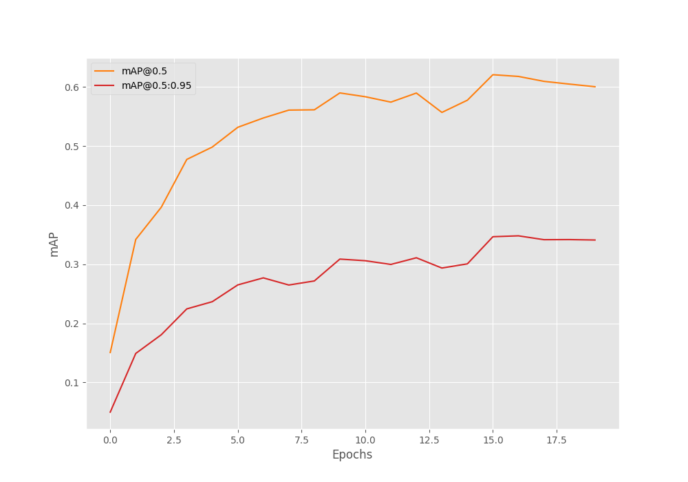
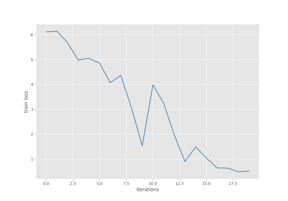
From the mAP graph, we can infer that the learning rate scheduler helped to boost the results a bit after epoch 15. With proper augmentations, we can improve the results further.
For now, we will move forward with the best model and carry out inference.
Inference Using the Trained DINOv3 Detection Model
First, we will carry out inference on images and then on videos using the trained model.
We need to execute the infer_det_image.py script to run the image inference.
python infer_det_image.py --input input/inference_data/images/ --model outputs/img_det/best_model.pth --model-name dinov3_convnext_tiny --config detection_configs/voc.yaml --threshold 0.15
The script accepts the path to the input images directory, the weights file, the model name, and the dataset configuration file. We have set a lower confidence threshold as our model is not very good at the moment. We can set a higher confidence threshold after training a better model.

There are a few observations to be made here. The model seems to be performing well when the scene is not too crowded. For example, in the case of the image with 4 women, the model detects only 3 of them. In another instance, the model seems to be failing to detect potted plants (top row, second image). In the final image, the model detects a few of the potted plants but fails to detect the sofas at all.
Let’s move on to video inference and analyze the performance. For this, we need to execute the infer_det_video.py script.
python infer_det_video.py --input input/inference_data/videos/video_5.mp4 --model outputs/img_det/best_model.pth --model-name dinov3_convnext_tiny --config detection_configs/voc.yaml --threshold 0.15
We can clearly see heavy flickering in the detections. This shows that the model needs more training to be confident in its detections. It recognizes the dog as a sheep in some instances as well. On an RTX 3080 GPU, we are getting an average of 72 FPS.
Summary and Conclusion
In this article, we tackled the problem of object detection by modifying the DINOv3 backbone and training it on the Pascal VOC dataset. The results are not perfect, but we do have a starting point. We covered the modeling, data, and training pipelines. There will be future articles after some substantial improvements to the codebase.
If you have any questions, thoughts, or suggestions, please leave them in the comment section. I will surely address them.
You can contact me using the Contact section. You can also find me on LinkedIn, and X.
