Image segmentation is one of the most important topics in the field of computer vision. A lot of research, time, and capital is being put into to create more efficient and real time image segmentation algorithms. And deep learning is a great helping hand in this process. In this article, we will take a look the concepts of image segmentation in deep learning.
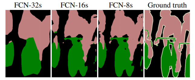
What will be learning in this article?
- What is image segmentation?
- Types of image segmentation in deep learning.
- Performance and evaluation metrics in deep learning image segmentation.
- Brief on some of the breakthrough papers in deep learning image segmentation.
- Real-life use cases of image segmentation in deep learning.
Note: This article is going to be theoretical. We will be discussing image segmentation in deep learning. This article is mainly to lay a groundwork for future articles where we will have lots of hands-on experimentation, discussing research papers in-depth, and implementing those papers as well.
What is Image Segmentation?
Before answering the question, let’s take a step back and discuss image classification a bit. If you are into deep learning, then you must be very familiar with image classification by now. In image classification, we use deep learning algorithms to classify a single image into one of the given classes. We do not account for the background or another object that is of less importance in the image context.
For example, take a look at the following image.
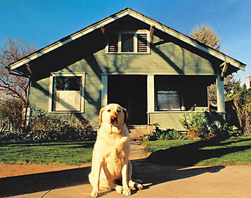
When we show the image to a deep learning image classification algorithm, then there is a very high chance that the algorithm will classify the image as that of a dog and completely ignore the house in the background.
Image Segmentation Comes into the Picture
Now, let’s say that we show the image to a deep learning based image segmentation algorithm. In this case, the deep learning model will try to classify each pixel of the image instead of the whole image. If everything works out, then the model will classify all the pixels making up the dog into one class. At the same time, it will classify all the pixels making up the house into another class. And if we are using some really good state-of-the-art algorithm, then it will also be able to classify the pixels of the grass and trees as well.
Then, there will be cases when the image will contain multiple objects with equal importance.
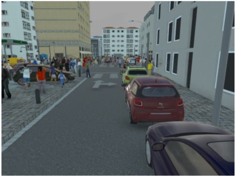
In figure 3, we have both people and cars in the image. It is obvious that a simple image classification algorithm will find it difficult to classify such an image. But what if we give this image as an input to a deep learning image segmentation algorithm? Well, we can expect the output something very similar to the following.
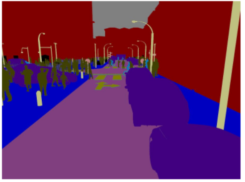
What you see in figure 4 is a typical output format from an image segmentation algorithm. Although it involves a lot of coding in the background, here is the breakdown:
- The deep learning model takes the input image.
- Then based on the classes it has been trained on, it will try to classify each pixel into one class.
- The output is then color coded so that we can easily distinguish one class from another.
- We can see that in figure 4, that all persons are coded into one color, the cars into another color, and the building into another color. If you observe closely, then you can see the segmentation model has also recognized the light poles and the road. This is really amazing.
Types of Image Segmentation
In this section, we will discuss the two categories of image segmentation in deep learning. They are:
- Semantic segmentation.
- Instance segmentation.
Semantic Segmentation
In semantic segmentation, we classify the objects belonging to the same class in the image with a single label. This means that when we visualize the output from the deep learning model, all the objects belonging to the same class are color coded with the same color.
For example, take the case where an image contains cars and buildings. In this image, we can color code all the pixels labeled as a car with red color and all the pixels labeled as building with the yellow color. Similarly, we will color code all the other pixels in the image.
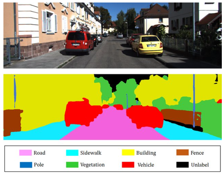
In figure 5, we can see that cars have a color code of red. This means all the pixels in the image which make up a car have a single label in the image. Similarly, all the buildings have a color code of yellow. The same is true for other classes such as road, fence, and vegetation.
You will notice that in the above image there is an unlabel category which has a black color. This means while writing the program we have not provided any label for the category and that will have a black color code. Mostly, in image segmentation this holds true for the background class. In some datasets is called background, some other datasets call it as void as well. These are mainly those areas in the image which are not of much importance and we can ignore them safely.
Instance Segmentation
In very simple words, instance segmentation is a combination of segmentation and object detection. But there are some particular differences of importance.
We now know that in semantic segmentation we label each pixel in an image into a single class. But in instance segmentation, we first detect an object in an image, when we apply a color coded mask around that object. And most probably, the color of each mask is different even if two objects belong to the same class.
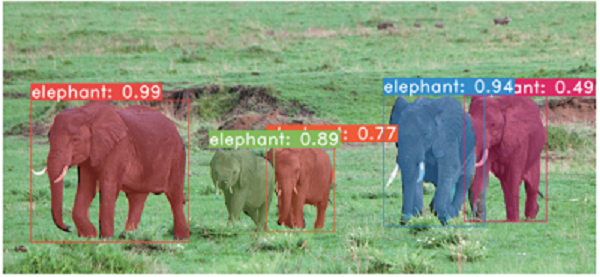
Figure 6 shows an example of instance segmentation from the YOLACT++ paper by Daniel Bolya, Chong Zhou, Fanyi Xiao, and Yong Jae Lee. Notice how all the elephants have a different color mask. Also, it is becoming more common for researchers nowadays to draw bounding boxes in instance segmentation. This makes the output more distinguishable.
Performance Evaluation Metrics for Image Segmentation in Deep Learning
Segmenting objects in images is alright, but how do we evaluate an image segmentation model?
In this section, we will discuss the various methods we can use to evaluate a deep learning segmentation model.
Many of the ideas here are taken from this amazing research survey – Image Segmentation Using Deep Learning: A Survey. This survey provides a lot of information on the different deep learning models and architectures for image segmentation over the years. This includes semantic segmentation, instance segmentation, and even medical imaging segmentation. If you have got a few hours to spare, do give the paper a read, you will surely learn a lot.
Now, let’s get back to the evaluation metrics in image segmentation.
Pixel Accuracy
Pixel accuracy is the ratio of the pixels that are classified to the total number of pixels in the image. Suppose that there are K + 1 classes in an image where K is the number of all the object classes, and one is the background class.
$$
Pixel\ Accuracy = \frac{\sum_{i=0}^{K}p_{ii}}{\sum_{i=0}^{K}\sum_{j=0}^{K}p_{ij}}
$$
In the above equation, \(p_{ij}\) are the pixels which belong to class \(i\) and are predicted as class \(j\).
Mean Pixel Accuracy
In mean pixel accuracy, the ratio of the correct pixels is computed in a per-class manner. Finally, the value is averaged over the total number of classes.
$$
Mean\ Pixel\ Accuracy =\frac{1}{K+1} \sum_{i=0}^{K}\frac{p_{ii}}{\sum_{j=0}^{K}p_{ij}}
$$
Intersection over Union (IoU) and Mean-IoU
IoU or otherwise known as the Jaccard Index is used for both object detection and image segmentation. It is the fraction of area of intersection of the predicted segmentation of map and the ground truth map, to the area of union of predicted and ground truth segmentation maps.
The following is the formula.
$$
IoU = \frac{|A \cap B|}{|A \cup B|}
$$
In the above formula, \(A\) and \(B\) are the predicted and ground truth segmentation maps respectively.
Coming to Mean IoU, it is perhaps one of the most widely used metric in code implementations and research paper implementations. It is the average of the IoU over all the classes.
Dice Coefficient and Dice Loss
The Dice coefficient is another popular evaluation metric in many modern research paper implementations of image segmentation.
It is a little it similar to the IoU metric. It is defined as the ratio of the twice the intersection of the predicted and ground truth segmentation maps to the total area of both the segmentation maps.
$$
Dice = \frac{2|A \cap B|}{|A| + |B|}
$$
Another metric that is becoming popular nowadays is the Dice Loss. Along with being a performance evaluation metric is also being used as the loss function while training the algorithm. For now, we will not go into much detail of the dice loss function. It is basically 1 – Dice Coefficient along with a few tweaks. The following is the formula.
$$
Dice\ Loss = 1- \frac{2|A \cap B| + Smooth}{|A| + |B| + Smooth}
$$
In the above function, the \(smooth\) constant has a few important functions. First of all, it avoids the division by zero error when calculating the loss. Secondly, in some particular cases, it can also reduce overfitting. We will perhaps discuss this in detail in one of the future tutorials, where we will implement the dice loss. For now, just keep the above formula in mind.
There are many other loss functions as well. If you are interested, you can read about them in this article. Also, if you are interested in metrics for object detection, then you can check one of my other articles here.
Some Great Papers on Deep Learning Image Segmentation
In this section, we will discuss some breakthrough papers in the field of image segmentation using deep learning. There are numerous papers regarding to image segmentation, easily spanning in hundreds. But we will discuss only four papers here, and that too briefly. To give proper justice to these papers, they require their own articles. Therefore, we will discuss just the important points here.
Fully Convolutional Networks for Image Segmentation
Fully Convolutional Networks for Semantic Segmentation by Jonathan Long, Evan Shelhamer, and Trevor Darrell was one of the breakthrough papers in the field of deep learning image segmentation.
Published in 2015, this became the state-of-the-art at the time. This image segmentation neural network model contains only convolutional layers and hence the name. The authors modified the GoogLeNet and VGG16 architectures by replacing the final fully connected layers with convolutional layers. This makes the network to output a segmentation map of the input image instead of the standard classification scores.
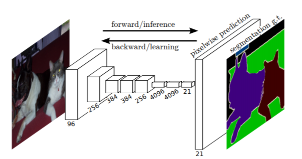
In the above figure (figure 7) you can see that the FCN model architecture contains only convolutional layers. The input is an RGB image and the output is a segmentation map. At the time of publication, the FCN methods achieved state-of-the-art results on many datasets including PASCAL VOC. But one major problem with the model was that it was very slow and could not be used for real-time segmentation. Most of the future segmentation models tried to address this issue.
SegNet
SegNet by Badrinarayanan et al. is a deep learning segmentation model based on the encoder-decoder architecture.

Take a look at figure 8. You can see that the trainable encoder network has 13 convolutional layers. These are the layers in the VGG16 network. The decoder network contains upsampling layers and convolutional layers. This decoder network is responsible for the pixel-wise classification of the input image and outputting the final segmentation map.
U-Net
U-Net by Ronneberger et al. is another segmentation model based on the encoder-decoder architecture.
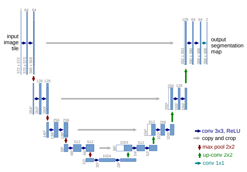
The U-Net mainly aims at segmenting medical images using deep learning techniques. The U-Net architecture comprises of two parts. One is the down-sampling network part that is an FCN-like network. The other one is the up-sampling part which increases the dimensions after each layer. This increase in dimensions leads to higher resolution segmentation maps which are a major requirement in medical imaging.
Mask-RCNN
The Mask-RCNN architecture for image segmentation is an extension of the Faster-RCNN object detection framework. The paper by Kaiming He, Georgia Gkioxari, Piotr Dollar, and Ross Girshick extends the Faster-RCNN object detector model to output both image segmentation masks and bounding box predictions as well.
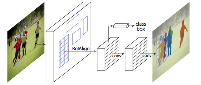
Figure 10 shows the network architecture for Mask-RCNN. The Mask-RCNN architecture contains three output branches. These include the branches for the bounding box coordinates, the output classes, and the segmentation map. The Mask-RCNN model combines the losses of all the three and trains the network jointly. At the time of publication (2015), the Mask-RCNN architecture beat all the previous benchmarks on the COCO dataset.
We will stop the discussion of deep learning segmentation models here. We did not cover many of the recent segmentation models. But we did cover some of the very important ones that paved the way for many state-of-the-art and real time segmentation models. We will discuss and implement many more deep learning segmentation models in future articles.
In the next section, we will discuss some real like application of deep learning based image segmentation.
Real-Life Use Cases and Applications of Image Segmentation in Deep Learning
In this final section of the tutorial about image segmentation, we will go over some of the real life applications of deep learning image segmentation techniques.
Medical Imaging
In my opinion, the best applications of deep learning are in the field of medical imaging. Starting from recognition to detection, to segmentation, the results are very positive.
Starting from segmenting tumors in brain and lungs to segmenting sites of pneumonia in lungs, image segmentation has been very helpful in medical imaging.
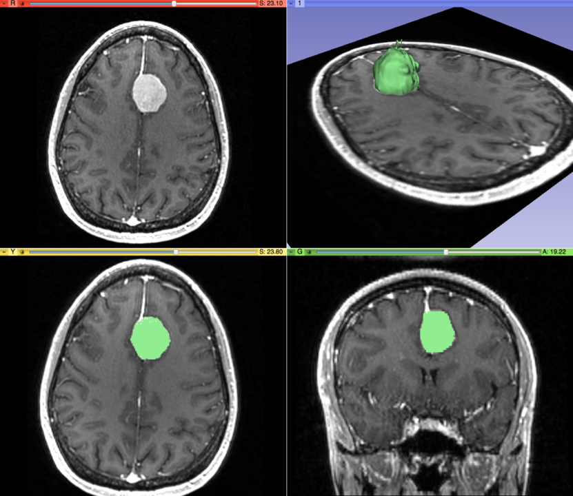
Figure 11 shows the 3D modeling and the segmentation of a meningeal tumor in the brain on the left hand side of the image. Segmenting the tumorous tissue makes it easier for doctors to analyze the severity of the tumor properly and hence, provide proper treatment.
We can also detect opacity in lungs caused due to pneumonia using deep learning object detection, and image segmentation.
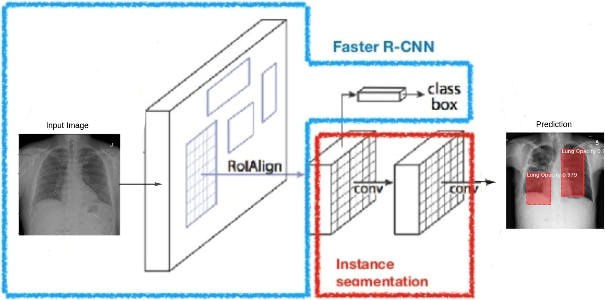
Figure 12 shows how a Faster RCNN based Mask RCNN model has been used to detect opacity in lungs. Such applications help doctors to identify critical and life-threatening diseases quickly and with ease.
Automous Driving
We know that it is only a matter of time before we see fleets of cars driving autonomously on roads. Many companies are investing large amounts of money to make autonomous driving a reality. And deep learning plays a very important role in that.
How does deep learning based image segmentation help here, you may ask. There are many usages.
Deep learning based image segmentation is used to segment lane lines on roads which help the autonomous cars to detect lane lines and align themselves correctly. Similarly, we can also use image segmentation to segment drivable lanes and areas on a road for vehicles.
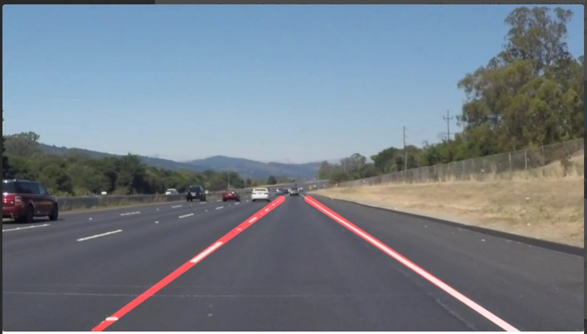
We can see that in figure 13 the lane marking has been segmented. Now, let’s take a look at the drivable area segmentation.
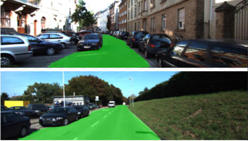
Figure 14 shows the segmented areas on the road where the vehicle can drive. Such segmentation helps autonomous vehicles to easily detect on which road they can drive and on which path they should drive.
Satellite Imaging
Satellite imaging is another area where image segmentation is being used widely.
Using image segmentation, we can detect roads, water bodies, trees, construction sites, and much more from a single satellite image. This problem is particularly difficult because the objects in a satellite image are very small.
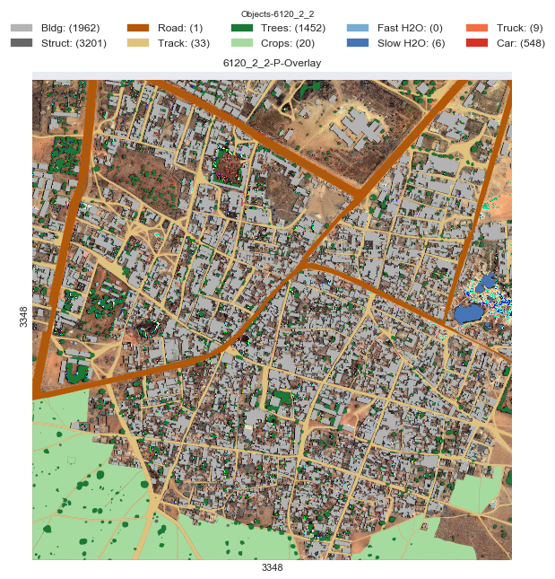
Figure 15 shows how image segmentation helps in satellite imaging and easily marking out different objects of interest. There are trees, crops, water bodies, roads, and even cars.
If you find the above image interesting and want to know more about it, then you can read this article.
Summary and Conclusion
In this article, you learned about image segmentation in deep learning. You got to know some of the breakthrough papers and the real life applications of deep learning. I hope that this provides a good starting point for you.
If you have any thoughts, ideas, or suggestions, then please leave them in the comment section. I will surely address them.
You can contact me using the Contact section. You can also find me on LinkedIn, and Twitter.



3 thoughts on “Introduction to Image Segmentation in Deep Learning”