

DINOv3 is the latest iteration in the DINO family of vision foundation models. It builds on the success of the previous DINOv2 and Web-DINO models. The authors have gone larger with the models – starting with a few million parameters to 7B parameters. Furthermore, the models have also been trained on a much larger dataset containing more than a billion images. All these lead to powerful backbones, which are suitable for downstream tasks, such as image classification. In this article, we will tackle image classification with DINOv3.
We will not go into the details provided in the official paper, which requires a dedicated article. Instead, we will focus more on the practical aspects, such as the models available, specifically the DINOv3 that we are choosing for image classification, and the task itself.
We will cover the following topics in image classification with DINOv3:
- Discussing the available DINOv3 models.
- The syntax and requirements to load a DINOv3 pretrained backbone.
- Exploring the GitHub repository that we will use for image classification with DINOv3.
- Tackling image classification training and inference.
What Are the Available DINOv3 Models?
The DINOv3 model was introduced in the paper by the same name by authors from Meta AI.
DINOv3 is available in 4 ConvNext and 6 Vision Transformer pretrained versions in their corresponding sizes.
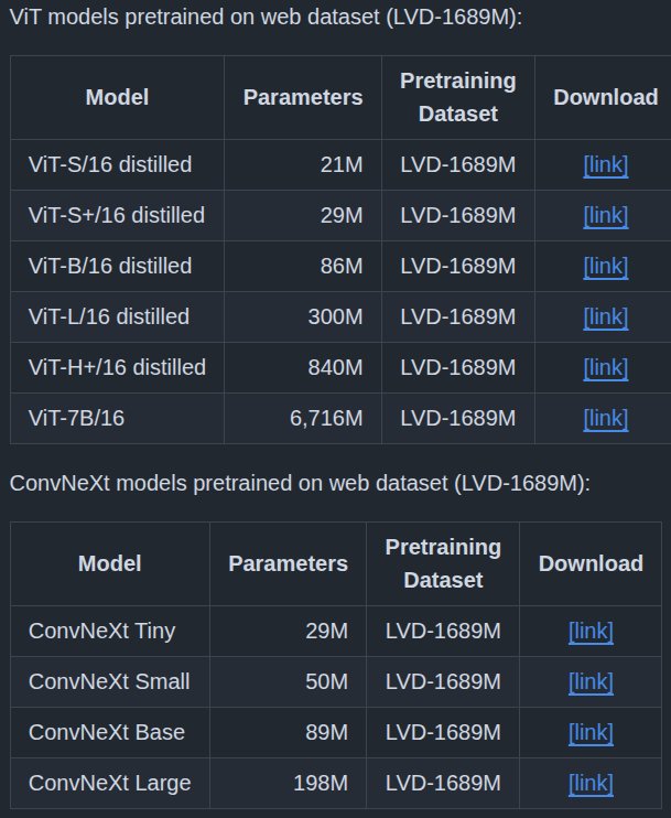
We will use the DINOv3 ViT-S/16 for image classification here.
How to Use the DINOv3 Models?
There are 2 prerequisites to loading a pretrained DINOv3 model.
First is cloning the official repository.
git clone https://github.com/facebookresearch/dinov3
Second is downloading the pretrained weights, for which we need to fill a form by clicking on one of the download links in the model table.
Following this, we can load the model using the following syntax.
model = torch.hub.load(
    'dinov3', # Path to the repository.
    'dinov3_vits16', # Name of the model.
    source='local',
    weights='dinov3_vits16_pretrain_lvd1689m-08c60483.pth' # Path to the corresponding weight file.
)
This first loads the model on the CPU, which we can then transfer to our device of choice.
The GitHub Repository That We Will Use for Training
I am maintaining a GitHub repository called DINOv3 stack that allows downstream tasks using DINOv3 backbones. Currently, it contains codebase for image classification and semantic segmentation. I will be adding code for object detection soon.
You can find dinov3_stack here.
You can explore the codebase before moving further. However, you do not need to clone it. The article comes with a zip file of the entire codebase to keep things from breaking when it is updated in the future.
The Dataset for Image Classification
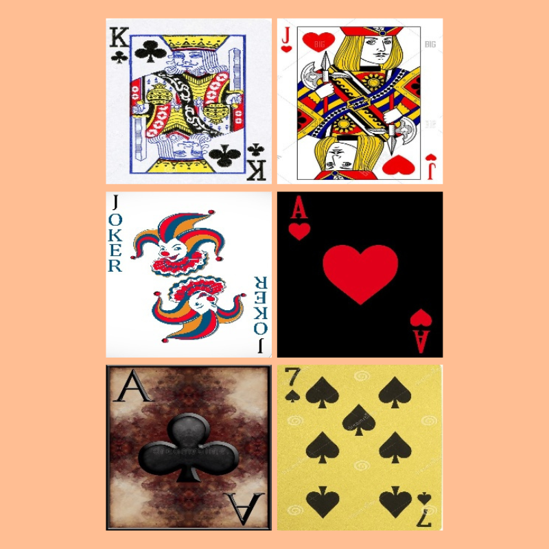
For the training experiments here, we will use a Card Image Classification dataset from Kaggle.
It’s an extremely high quality dataset and possibly without any mistakes. There are 7624 training, 265 validation, and 265 test images across 53 classes – one class for each card type. The entire dataset is present in PyTorch ImageFolder structure, which makes things easier for us.
Here are some samples from the training set.
Here is the directory structure after downloading and extracting it.
├── 14card types-14-(200 X 200)-94.61.h5
├── 53cards-53-(200 X 200)-100.00.h5
├── cards.csv
├── test  [53 entries exceeds filelimit, not opening dir]
├── train  [53 entries exceeds filelimit, not opening dir]
└── valid  [53 entries exceeds filelimit, not opening dir]
There are three folders for the three splits. It also comes with pretrained TensorFlow models and a CSV file that we can ignore.
This dataset is just perfect for our experiments. It is difficult enough to explore the difference between fine-tuning the backbone layers and transfer learning while keeping the backbone frozen.
Project Directory Structure
Let’s check the project directory structure.
├── classification_configs
│   ├── cards.yaml
│   └── leaf_disease.yaml
├── dinov3
│   ├── dinov3
│   ├── notebooks
│   ├── __pycache__
│   ├── CODE_OF_CONDUCT.md
│   ├── conda.yaml
│   ├── CONTRIBUTING.md
│   ├── hubconf.py
│   ├── LICENSE.md
│   ├── MODEL_CARD.md
│   ├── pyproject.toml
│   ├── README.md
│   ├── requirements-dev.txt
│   ├── requirements.txt
│   └── setup.py
├── input
│   ├── archive
│   │   ├── test
│   │   ├── train
│   │   ├── valid
│   │   ├── 14card types-14-(200 X 200)-94.61.h5
│   │   ├── 53cards-53-(200 X 200)-100.00.h5
│   │   └── cards.csv
│   ├── inference_data
│   │   ├── ace_of_clubs.jpg
│   │   ├── ace_of_diamonds.jpg
│   │   ├── jack_of_clubs.jpg
│   │   └── two_of_spades.jpg
│   ├── archive.zip
│   └── readme.txt
├── outputs
│   ├── fine_tune
│   ├── inference_results
│   └── transfer_learn
├── segmentation_configs
│   ├── person.yaml
│   └── voc.yaml
├── src
│   ├── img_cls
│   └── img_seg
├── weights
│   └── dinov3_vits16_pretrain_lvd1689m-08c60483.pth
├── infer_classifier.py
├── infer_seg_image.py
├── infer_seg_video.py
├── License
├── NOTES.md
├── README.md
├── requirements.txt
├── train_classifier.py
└── train_segmentation.py
Here are a few important pointers:
- We add the
dinov3GitHub repository as a submodule to the project directory so that we can load the models. - The
srcdirectory contains all the task specific source code files. - The card classification dataset is present in the
input/archivefolder after extracting it. We also have ainference_datafolder with a few images from the test set. - As we need the pretrained weights, it is present in the
weightsdirectory. - The parent project directory contains the
train_classifier.pyfile that is the executable script to start the image classification training. We also have inference scripts in the parent folder. - The
outputsdirectory contains the fine-tuned models after the training experiments.
We will go through the rest of the necessary files and folders as we need them.
All the dinov3_stack code files, fine-tuned weights, and inference data are available to download via the download section.
Download Code
Prerequisites
Dataset structure:
After downloading and extracting the codebase, make sure that you download the dataset from Kaggle and arrange it in the above structure.
Adding DINOv3 repository as submodule:
Next, we need to initialize the DINOv3 repository as a submodule. Execute the following command within the downloaded project folder after extracting it.
git submodule update --init
Creating a weights directory and keeping the DINOv3-ViT-S weights:
Create a weights directory and keep the DINOv3 ViT-S/16 weight file in it after filling the form and downloading it. The downloaded file should have a name similar to dinov3_vits16_pretrain_lvd1689m-08c60483.pth
Install the dependencies:
Now, install the libraries needed.
pip install -r requirements.txt
This completes all the setup we need.
More articles on DINO models that might be useful:
- Image Classification with Web-DINO
- Semantic Segmentation using Web-DINO
- Pretraining DINOv2 for Semantic Segmentation
- Multi-Class Semantic Segmentation using DINOv2
- DINOv2 Segmentation – Fine-Tuning and Transfer Learning Experiments
Image Classification with DINOv3
Let’s jump into the coding part of the article. We will start with the exploration of creating an image classification model using the DINOv3 backbone, then move to training and inference.
Image Classification Model Using DINOv3 Backbone
The code for the model creation is present in src/img_cls/model.py file.
There are two steps to creating the model:
- First is loading the pretrained backbone.
- Second is adding a simple Linear Classifier head on top of it.
The following code block contains the code to load the pretrained backbone.
"""
Building a linear classifier on top of DINOv3 backbone.
"""

import torch

from collections import OrderedDict

def load_model(weights: str=None, model_name: str=None, repo_dir: str=None):
    if weights is not None:
        print('Loading pretrained backbone weights from: ', weights)
        model = torch.hub.load(
            repo_dir,
            model_name,
            source='local',
            weights=weights
        )
    else:
        print('No pretrained weights path given. Loading with random weights.')
        model = torch.hub.load(
            repo_dir,
            model_name,
            source='local'
        )

    return model
The load_model function accepts the pretrained weights, the mode name, and the repository path as parameters.
The syntax for loading the backbone model is similar to what we saw earlier.
Next, we have the build_model function to create the final model.
def build_model(
    num_classes: int=10,
    fine_tune: bool=False,
    weights: str=None,
    model_name: str=None,
    repo_dir: str=None
):
    backbone_model = load_model(
        weights=weights, model_name=model_name, repo_dir=repo_dir
    )

    model = torch.nn.Sequential(OrderedDict([
        ('backbone', backbone_model),
        ('head', torch.nn.Linear(
            in_features=backbone_model.norm.normalized_shape[0],
            out_features=num_classes,
            bias=True
        ))
    ]))

    if not fine_tune:
        for params in model.backbone.parameters():
            params.requires_grad = False

    return model
After loading the backbone, we create a Sequential ordered dictionary consisting of the backbone and a simple Linear Classifier with the specified number of classes. It is an extremely simple image classification mode, just as described in the official paper.
We have a fine_tune argument to control whether we want to update the weights of the backbone or not.
The file also has a main block for sanity checking.
if __name__ == '__main__':
    from PIL import Image
    from torchvision import transforms
    from torchinfo import summary

    import numpy as np

    # We can give any multiple of 14.
    sample_size = 224

    # Define image transformation
    transform = transforms.Compose([
        transforms.Resize(
            sample_size,
            interpolation=transforms.InterpolationMode.BICUBIC
        ),
        transforms.CenterCrop(sample_size),
        transforms.ToTensor(),
        transforms.Normalize(
            mean=(0.485, 0.456, 0.406),
            std=(0.229, 0.224, 0.225)
        )
    ])

    # Loading the pretrained model without classification head.
    model = load_model(model_name='dinov3_vits16', repo_dir='dinov3')

    # Total parameters and trainable parameters.
    total_params = sum(p.numel() for p in model.parameters())
    print(f"{total_params:,} total parameters.")
    total_trainable_params = sum(
        p.numel() for p in model.parameters() if p.requires_grad)
    print(f"{total_trainable_params:,} training parameters.")

    # Testing forward pass.
    pil_image = Image.fromarray(np.ones((sample_size, sample_size, 3), dtype=np.uint8))
    model_input = transform(pil_image).unsqueeze(0)

    summary(
        model,
        input_data=model_input,
        col_names=('input_size', 'output_size', 'num_params'),
        row_settings=['var_names']
    )

    # Manual torch forward pass.
    with torch.no_grad():
        features = model.forward_features(model_input)
        patch_features = features['x_norm_patchtokens']

    print(features.keys())
    print(f"Patch features shape: {patch_features.shape}")

    # Check the forward passes through the complete model.
    # To check what gets fed to the classification layer.
    model_cls = build_model(model_name='dinov3_vits16', repo_dir='dinov3')
    features = model_cls.backbone(model_input)
    print(f"Shape of features getting fed to classification layer: {features.shape}")
Executing the file gives the following output.
python src/img_cls/model.py
No pretrained weights path given. Loading with random weights. 21,601,152 total parameters. 21,601,152 training parameters. ============================================================================================================================= Layer (type (var_name)) Input Shape Output Shape Param # ============================================================================================================================= DinoVisionTransformer (DinoVisionTransformer) [1, 3, 224, 224] [1, 384] 2,304 ├─PatchEmbed (patch_embed) [1, 3, 224, 224] [1, 14, 14, 384] -- │ └─Conv2d (proj) [1, 3, 224, 224] [1, 384, 14, 14] 295,296 │ └─Identity (norm) [1, 196, 384] [1, 196, 384] -- ├─RopePositionEmbedding (rope_embed) -- [196, 64] -- ├─ModuleList (blocks) -- -- (recursive) │ └─SelfAttentionBlock (0) [1, 201, 384] [1, 201, 384] -- │ │ └─LayerNorm (norm1) [1, 201, 384] [1, 201, 384] 768 │ │ └─SelfAttention (attn) [1, 201, 384] [1, 201, 384] 591,360 │ │ └─LayerScale (ls1) [1, 201, 384] [1, 201, 384] 384 │ │ └─LayerNorm (norm2) [1, 201, 384] [1, 201, 384] 768 │ │ └─Mlp (mlp) [1, 201, 384] [1, 201, 384] 1,181,568 │ │ └─LayerScale (ls2) [1, 201, 384] [1, 201, 384] 384 ├─RopePositionEmbedding (rope_embed) -- [196, 64] -- ├─ModuleList (blocks) -- -- (recursive) │ └─SelfAttentionBlock (1) [1, 201, 384] [1, 201, 384] -- │ │ └─LayerNorm (norm1) [1, 201, 384] [1, 201, 384] 768 │ │ └─SelfAttention (attn) [1, 201, 384] [1, 201, 384] 591,360 │ │ └─LayerScale (ls1) [1, 201, 384] [1, 201, 384] 384 │ │ └─LayerNorm (norm2) [1, 201, 384] [1, 201, 384] 768 │ │ └─Mlp (mlp) [1, 201, 384] [1, 201, 384] 1,181,568 │ │ └─LayerScale (ls2) [1, 201, 384] [1, 201, 384] 384 ├─RopePositionEmbedding (rope_embed) -- [196, 64] -- ├─ModuleList (blocks) -- -- (recursive) │ └─SelfAttentionBlock (2) [1, 201, 384] [1, 201, 384] -- │ │ └─LayerNorm (norm1) [1, 201, 384] [1, 201, 384] 768 │ │ └─SelfAttention (attn) [1, 201, 384] [1, 201, 384] 591,360 │ │ └─LayerScale (ls1) [1, 201, 384] [1, 201, 384] 384 │ │ └─LayerNorm (norm2) [1, 201, 384] [1, 201, 384] 768 │ │ └─Mlp (mlp) [1, 201, 384] [1, 201, 384] 1,181,568 │ │ └─LayerScale (ls2) [1, 201, 384] [1, 201, 384] 384 ├─RopePositionEmbedding (rope_embed) -- [196, 64] -- ├─ModuleList (blocks) -- -- (recursive) │ └─SelfAttentionBlock (3) [1, 201, 384] [1, 201, 384] -- │ │ └─LayerNorm (norm1) [1, 201, 384] [1, 201, 384] 768 │ │ └─SelfAttention (attn) [1, 201, 384] [1, 201, 384] 591,360 │ │ └─LayerScale (ls1) [1, 201, 384] [1, 201, 384] 384 │ │ └─LayerNorm (norm2) [1, 201, 384] [1, 201, 384] 768 │ │ └─Mlp (mlp) [1, 201, 384] [1, 201, 384] 1,181,568 │ │ └─LayerScale (ls2) [1, 201, 384] [1, 201, 384] 384 ├─RopePositionEmbedding (rope_embed) -- [196, 64] -- ├─ModuleList (blocks) -- -- (recursive) │ └─SelfAttentionBlock (4) [1, 201, 384] [1, 201, 384] -- │ │ └─LayerNorm (norm1) [1, 201, 384] [1, 201, 384] 768 │ │ └─SelfAttention (attn) [1, 201, 384] [1, 201, 384] 591,360 │ │ └─LayerScale (ls1) [1, 201, 384] [1, 201, 384] 384 │ │ └─LayerNorm (norm2) [1, 201, 384] [1, 201, 384] 768 │ │ └─Mlp (mlp) [1, 201, 384] [1, 201, 384] 1,181,568 │ │ └─LayerScale (ls2) [1, 201, 384] [1, 201, 384] 384 ├─RopePositionEmbedding (rope_embed) -- [196, 64] -- ├─ModuleList (blocks) -- -- (recursive) │ └─SelfAttentionBlock (5) [1, 201, 384] [1, 201, 384] -- │ │ └─LayerNorm (norm1) [1, 201, 384] [1, 201, 384] 768 │ │ └─SelfAttention (attn) [1, 201, 384] [1, 201, 384] 591,360 │ │ └─LayerScale (ls1) [1, 201, 384] [1, 201, 384] 384 │ │ └─LayerNorm (norm2) [1, 201, 384] [1, 201, 384] 768 │ │ └─Mlp (mlp) [1, 201, 384] [1, 201, 384] 1,181,568 │ │ └─LayerScale (ls2) [1, 201, 384] [1, 201, 384] 384 ├─RopePositionEmbedding (rope_embed) -- [196, 64] -- ├─ModuleList (blocks) -- -- (recursive) │ └─SelfAttentionBlock (6) [1, 201, 384] [1, 201, 384] -- │ │ └─LayerNorm (norm1) [1, 201, 384] [1, 201, 384] 768 │ │ └─SelfAttention (attn) [1, 201, 384] [1, 201, 384] 591,360 │ │ └─LayerScale (ls1) [1, 201, 384] [1, 201, 384] 384 │ │ └─LayerNorm (norm2) [1, 201, 384] [1, 201, 384] 768 │ │ └─Mlp (mlp) [1, 201, 384] [1, 201, 384] 1,181,568 │ │ └─LayerScale (ls2) [1, 201, 384] [1, 201, 384] 384 ├─RopePositionEmbedding (rope_embed) -- [196, 64] -- ├─ModuleList (blocks) -- -- (recursive) │ └─SelfAttentionBlock (7) [1, 201, 384] [1, 201, 384] -- │ │ └─LayerNorm (norm1) [1, 201, 384] [1, 201, 384] 768 │ │ └─SelfAttention (attn) [1, 201, 384] [1, 201, 384] 591,360 │ │ └─LayerScale (ls1) [1, 201, 384] [1, 201, 384] 384 │ │ └─LayerNorm (norm2) [1, 201, 384] [1, 201, 384] 768 │ │ └─Mlp (mlp) [1, 201, 384] [1, 201, 384] 1,181,568 │ │ └─LayerScale (ls2) [1, 201, 384] [1, 201, 384] 384 ├─RopePositionEmbedding (rope_embed) -- [196, 64] -- ├─ModuleList (blocks) -- -- (recursive) │ └─SelfAttentionBlock (8) [1, 201, 384] [1, 201, 384] -- │ │ └─LayerNorm (norm1) [1, 201, 384] [1, 201, 384] 768 │ │ └─SelfAttention (attn) [1, 201, 384] [1, 201, 384] 591,360 │ │ └─LayerScale (ls1) [1, 201, 384] [1, 201, 384] 384 │ │ └─LayerNorm (norm2) [1, 201, 384] [1, 201, 384] 768 │ │ └─Mlp (mlp) [1, 201, 384] [1, 201, 384] 1,181,568 │ │ └─LayerScale (ls2) [1, 201, 384] [1, 201, 384] 384 ├─RopePositionEmbedding (rope_embed) -- [196, 64] -- ├─ModuleList (blocks) -- -- (recursive) │ └─SelfAttentionBlock (9) [1, 201, 384] [1, 201, 384] -- │ │ └─LayerNorm (norm1) [1, 201, 384] [1, 201, 384] 768 │ │ └─SelfAttention (attn) [1, 201, 384] [1, 201, 384] 591,360 │ │ └─LayerScale (ls1) [1, 201, 384] [1, 201, 384] 384 │ │ └─LayerNorm (norm2) [1, 201, 384] [1, 201, 384] 768 │ │ └─Mlp (mlp) [1, 201, 384] [1, 201, 384] 1,181,568 │ │ └─LayerScale (ls2) [1, 201, 384] [1, 201, 384] 384 ├─RopePositionEmbedding (rope_embed) -- [196, 64] -- ├─ModuleList (blocks) -- -- (recursive) │ └─SelfAttentionBlock (10) [1, 201, 384] [1, 201, 384] -- │ │ └─LayerNorm (norm1) [1, 201, 384] [1, 201, 384] 768 │ │ └─SelfAttention (attn) [1, 201, 384] [1, 201, 384] 591,360 │ │ └─LayerScale (ls1) [1, 201, 384] [1, 201, 384] 384 │ │ └─LayerNorm (norm2) [1, 201, 384] [1, 201, 384] 768 │ │ └─Mlp (mlp) [1, 201, 384] [1, 201, 384] 1,181,568 │ │ └─LayerScale (ls2) [1, 201, 384] [1, 201, 384] 384 ├─RopePositionEmbedding (rope_embed) -- [196, 64] -- ├─ModuleList (blocks) -- -- (recursive) │ └─SelfAttentionBlock (11) [1, 201, 384] [1, 201, 384] -- │ │ └─LayerNorm (norm1) [1, 201, 384] [1, 201, 384] 768 │ │ └─SelfAttention (attn) [1, 201, 384] [1, 201, 384] 591,360 │ │ └─LayerScale (ls1) [1, 201, 384] [1, 201, 384] 384 │ │ └─LayerNorm (norm2) [1, 201, 384] [1, 201, 384] 768 │ │ └─Mlp (mlp) [1, 201, 384] [1, 201, 384] 1,181,568 │ │ └─LayerScale (ls2) [1, 201, 384] [1, 201, 384] 384 ├─LayerNorm (norm) [1, 201, 384] [1, 201, 384] 768 ├─Identity (head) [1, 384] [1, 384] -- ============================================================================================================================= Total params: 21,601,152 Trainable params: 21,601,152 Non-trainable params: 0 Total mult-adds (Units.MEGABYTES): 79.17 ============================================================================================================================= Input size (MB): 0.60 Forward/backward pass size (MB): 97.55 Params size (MB): 86.40 Estimated Total Size (MB): 184.54 ============================================================================================================================= dict_keys(['x_norm_clstoken', 'x_storage_tokens', 'x_norm_patchtokens', 'x_prenorm', 'masks']) Patch features shape: torch.Size([1, 196, 384]) No pretrained weights path given. Loading with random weights. Shape of features getting fed to classification layer: torch.Size([1, 384])
The smallest DINOv3 Transformer model contains around 21.6 million parameters and outputs a feature of shape [batch_size, embedding_dim] from the final layer.
This is all about the model creation that we need to know.
The Dataset Preparation Steps
The details of the dataset preparation are present in src/img_cls/datasets.py. Although we will not go into the coding details, here are some important pointers:
- We resize the images to 256×256 resolution and center crop them to 224×224 resolution.
- As per the DINOv3 paper, we apply the ImageNet mean and standard deviation during normalization.
- For training, at the moment, we are applying just the horizontal flipping augmentation.
Utility Scripts
The code in src/img_cls/utils.py contains utility and helper functions such as:
- Saving the model weights according to the best loss.
- Plotting accuracy and loss graphs.
Starting the Training
All the training and inference experiments were carried out on a system with 10GB RTX 3080 GPU, 32GB RAM, and 10th generation i7 CPU.
The train_classifier.py file in the parent directory is the executable script. It supports a number of command line arguments. However, we will go through the ones that we use during training. We will carry out two experiments, one where we keep the backbone frozen, and the other where we train the entire model. This will give us a good comparison between transfer learning and fine-tuning.
Transfer Learning with Frozen Backbone
Let’s start the transfer learning process while keeping the backbone frozen.
python train_classifier.py --train-dir input/archive/train/ --valid-dir input/archive/valid/ --weights weights/dinov3_vits16_pretrain_lvd1689m-08c60483.pth --repo-dir dinov3 --model-name dinov3_vits16 --epochs 80 --out-dir transfer_learn -lr 0.005
--train-dirand--valid-dir: These two arguments expect the path to the PyTorch ImageFolder structure dataset directories.--weights: The path to the weights file for loading the pretrained backbone. It can either be an absolute path or a relative path from where we are executing the script.--repo-dir: Path to the cloned DINOv3 repository. It can either be an absolute path or a relative path from where we are executing the script.--epochs: We are training for 80 epochs here.--out-dir: Name of the subdirectory to save the results inside theoutputsdirectory.-lr: The learning rate. As the default batch size is 32, and we are freezing the backbone here, we can use a high learning rate.--model-name: The DINOv3 model that we want to load.
Here are the truncated training logs.
Loading pretrained backbone weights from:  weights/dinov3_vits16_pretrain_lvd1689m-08c60483.pth
Sequential(
  (backbone): DinoVisionTransformer(
    (patch_embed): PatchEmbed(
      (proj): Conv2d(3, 384, kernel_size=(16, 16), stride=(16, 16))
      (norm): Identity()
    )
    (rope_embed): RopePositionEmbedding()
    (blocks): ModuleList(
      (0-11): 12 x SelfAttentionBlock(
        (norm1): LayerNorm((384,), eps=1e-05, elementwise_affine=True)
        (attn): SelfAttention(
          (qkv): LinearKMaskedBias(in_features=384, out_features=1152, bias=True)
          (attn_drop): Dropout(p=0.0, inplace=False)
          (proj): Linear(in_features=384, out_features=384, bias=True)
          (proj_drop): Dropout(p=0.0, inplace=False)
        )
        (ls1): LayerScale()
        (norm2): LayerNorm((384,), eps=1e-05, elementwise_affine=True)
        (mlp): Mlp(
          (fc1): Linear(in_features=384, out_features=1536, bias=True)
          (act): GELU(approximate='none')
          (fc2): Linear(in_features=1536, out_features=384, bias=True)
          (drop): Dropout(p=0.0, inplace=False)
        )
        (ls2): LayerScale()
      )
    )
    (norm): LayerNorm((384,), eps=1e-05, elementwise_affine=True)
    (head): Identity()
  )
  (head): Linear(in_features=384, out_features=53, bias=True)
)
21,621,557 total parameters.
20,405 training parameters.
[INFO]: Epoch 1 of 80
Training
100%|██████████████████████████████████████████████████████████████████████████████████████████████████████████████████████████████████████████████████████| 239/239 [00:09<00:00, 26.10it/s]
Validation
100%|██████████████████████████████████████████████████████████████████████████████████████████████████████████████████████████████████████████████████████████| 9/9 [00:00<00:00, 23.11it/s]
Training loss: 3.192, training acc: 22.875
Validation loss: 2.546, validation acc: 40.755

Best validation loss: 2.546049462424384

Saving best model for epoch: 1

--------------------------------------------------
.
.
.
LR for next epoch: [0.005]
[INFO]: Epoch 78 of 80
Training
100%|██████████████████████████████████████████████████████████████████████████████████████████████████████████████████████████████████████████████████████| 239/239 [00:09<00:00, 26.39it/s]
Validation
100%|██████████████████████████████████████████████████████████████████████████████████████████████████████████████████████████████████████████████████████████| 9/9 [00:00<00:00, 22.86it/s]
Training loss: 0.579, training acc: 87.907
Validation loss: 0.907, validation acc: 73.962

Best validation loss: 0.9065513677067227

Saving best model for epoch: 78

--------------------------------------------------.
.
.
.
LR for next epoch: [0.005]
[INFO]: Epoch 80 of 80
Training
100%|██████████████████████████████████████████████████████████████████████████████████████████████████████████████████████████████████████████████████████| 239/239 [00:09<00:00, 26.53it/s]
Validation
100%|██████████████████████████████████████████████████████████████████████████████████████████████████████████████████████████████████████████████████████████| 9/9 [00:00<00:00, 23.33it/s]
Training loss: 0.580, training acc: 87.303
Validation loss: 0.913, validation acc: 75.094
--------------------------------------------------
LR for next epoch: [0.005]
TRAINING COMPLETE
As we can see, our Linear Classifier head contributed to just 20,405 trainable parameters. This is great for resource constrained and faster training. However, even after 80 epochs, we have the best validation accuracy of only around 74%. Here are the graphs.
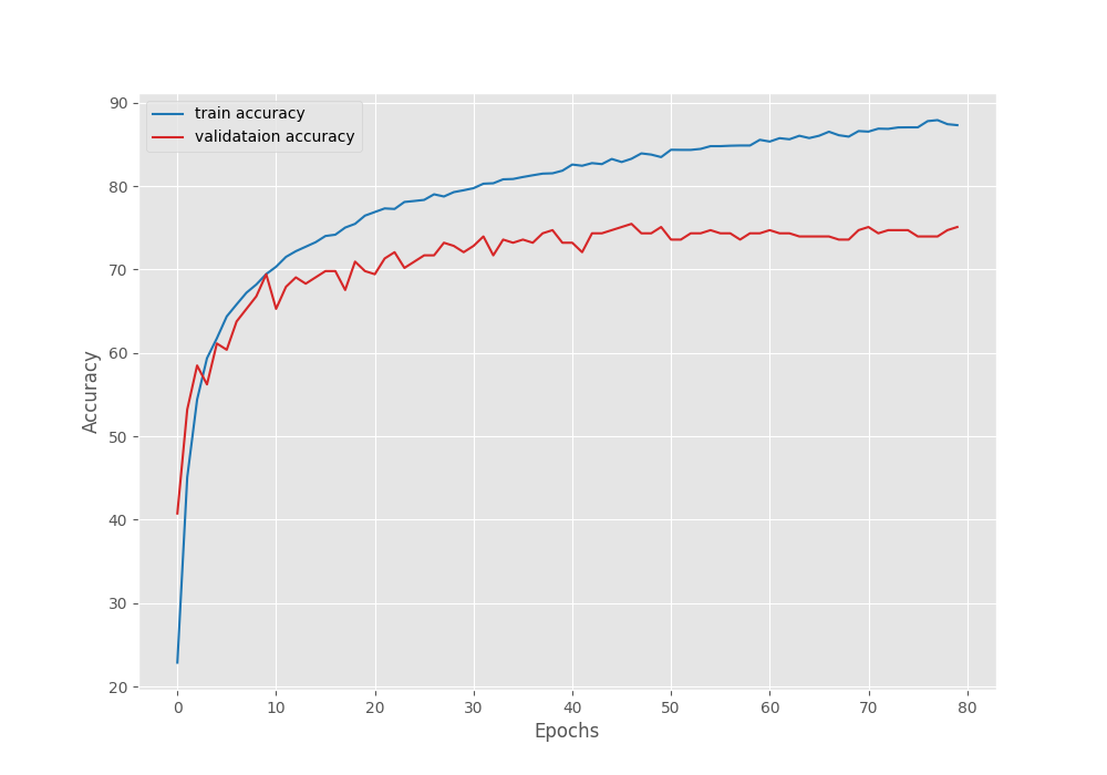
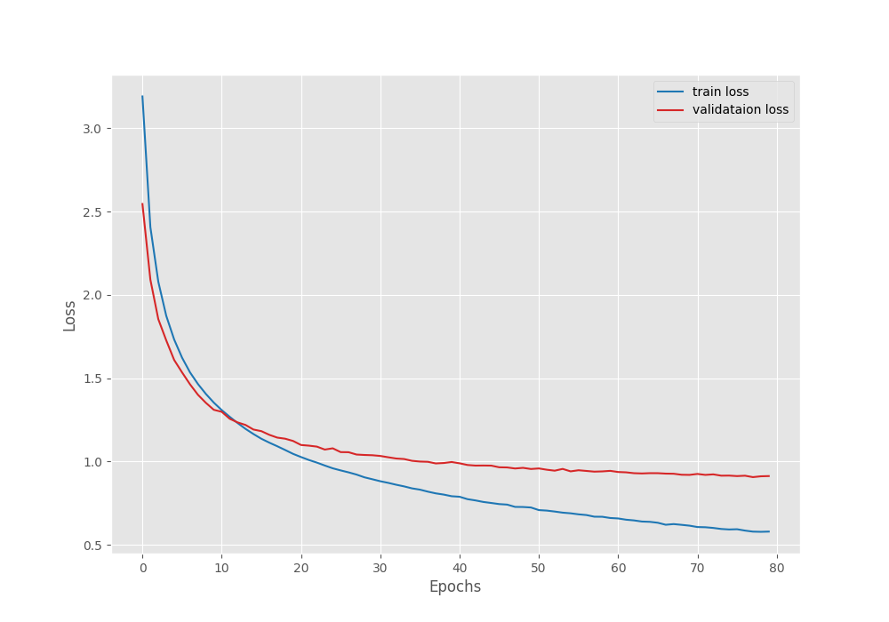
We can see that the validation accuracy line shows overfitting. Even if we use a learning rate scheduler and train for longer, it will not improve a lot, although that is subject to experiment.
Fine-Tuning the Backbone
Let’s move to the second phase of our experiments, fine-tuning the entire DINOv3 model for image classification.
python train_classifier.py --train-dir input/archive/train/ --valid-dir input/archive/valid/ --weights weights/dinov3_vits16_pretrain_lvd1689m-08c60483.pth --repo-dir dinov3 --model-name dinov3_vits16 --epochs 20 --fine-tune --out-dir fine_tune
This time, we are training for 20 epochs while keeping the rest of the parameters the same. We use an additional boolean fine_tune command line argument, which tells the script to make the backbone trainable.
Here are the logs.
Loading pretrained backbone weights from:  weights/dinov3_vits16_pretrain_lvd1689m-08c60483.pth
Sequential(
  (backbone): DinoVisionTransformer(
    (patch_embed): PatchEmbed(
      (proj): Conv2d(3, 384, kernel_size=(16, 16), stride=(16, 16))
      (norm): Identity()
    )
    (rope_embed): RopePositionEmbedding()
    (blocks): ModuleList(
      (0-11): 12 x SelfAttentionBlock(
        (norm1): LayerNorm((384,), eps=1e-05, elementwise_affine=True)
        (attn): SelfAttention(
          (qkv): LinearKMaskedBias(in_features=384, out_features=1152, bias=True)
          (attn_drop): Dropout(p=0.0, inplace=False)
          (proj): Linear(in_features=384, out_features=384, bias=True)
          (proj_drop): Dropout(p=0.0, inplace=False)
        )
        (ls1): LayerScale()
        (norm2): LayerNorm((384,), eps=1e-05, elementwise_affine=True)
        (mlp): Mlp(
          (fc1): Linear(in_features=384, out_features=1536, bias=True)
          (act): GELU(approximate='none')
          (fc2): Linear(in_features=1536, out_features=384, bias=True)
          (drop): Dropout(p=0.0, inplace=False)
        )
        (ls2): LayerScale()
      )
    )
    (norm): LayerNorm((384,), eps=1e-05, elementwise_affine=True)
    (head): Identity()
  )
  (head): Linear(in_features=384, out_features=53, bias=True)
)
21,621,557 total parameters.
21,621,557 training parameters.
[INFO]: Epoch 1 of 20
Training
100%|██████████████████████████████████████████████████████████████████████████████████████████████████████████████████████████████████████████████████████| 239/239 [00:25<00:00,  9.53it/s]
Validation
100%|██████████████████████████████████████████████████████████████████████████████████████████████████████████████████████████████████████████████████████████| 9/9 [00:00<00:00, 22.58it/s]
Training loss: 3.494, training acc: 14.507
Validation loss: 2.790, validation acc: 27.925

Best validation loss: 2.789550463358561

Saving best model for epoch: 1

--------------------------------------------------
.
.
.
LR for next epoch: [0.001]
[INFO]: Epoch 20 of 20
Training
100%|██████████████████████████████████████████████████████████████████████████████████████████████████████████████████████████████████████████████████████| 239/239 [00:25<00:00,  9.49it/s]
Validation
100%|██████████████████████████████████████████████████████████████████████████████████████████████████████████████████████████████████████████████████████████| 9/9 [00:00<00:00, 21.50it/s]
Training loss: 0.064, training acc: 99.567
Validation loss: 0.161, validation acc: 97.358

Best validation loss: 0.16083565312955114

Saving best model for epoch: 20

--------------------------------------------------
LR for next epoch: [0.001]
TRAINING COMPLETE
This time, the model kept improving till the end of the training. We have the best validation loss of 0.16 and validation accuracy of 97.35%.
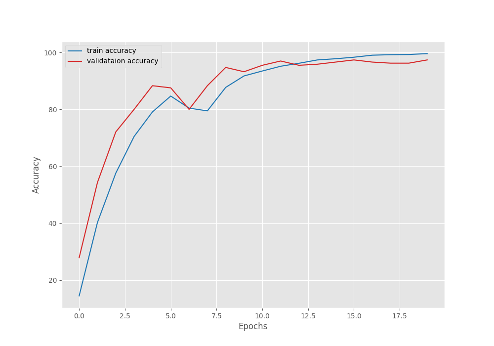
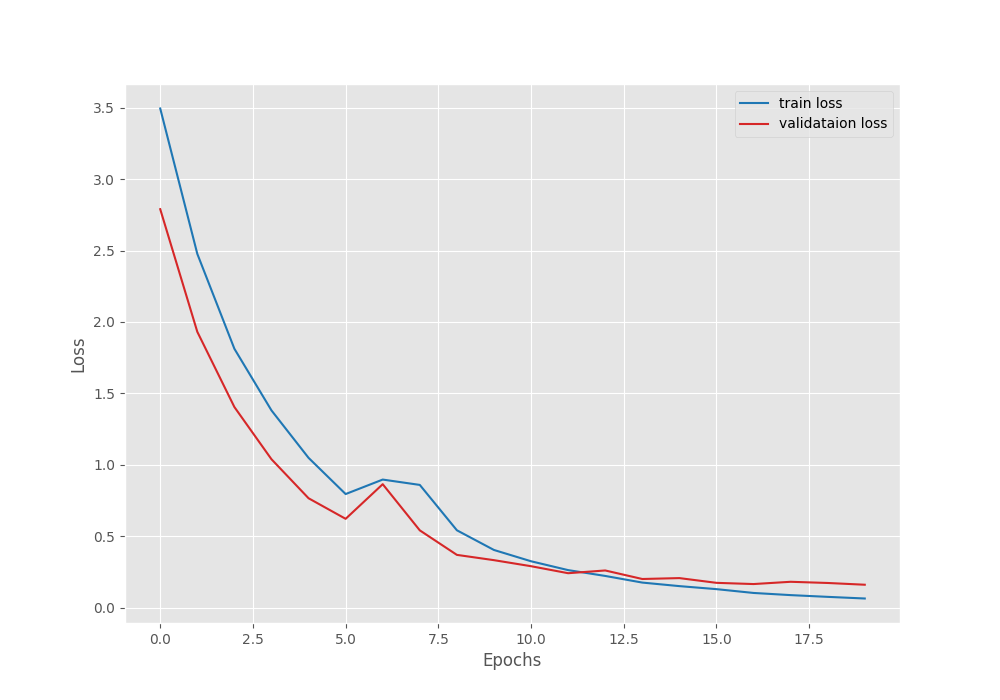
Training for longer, along with a learning rate scheduler, might help more in this case.
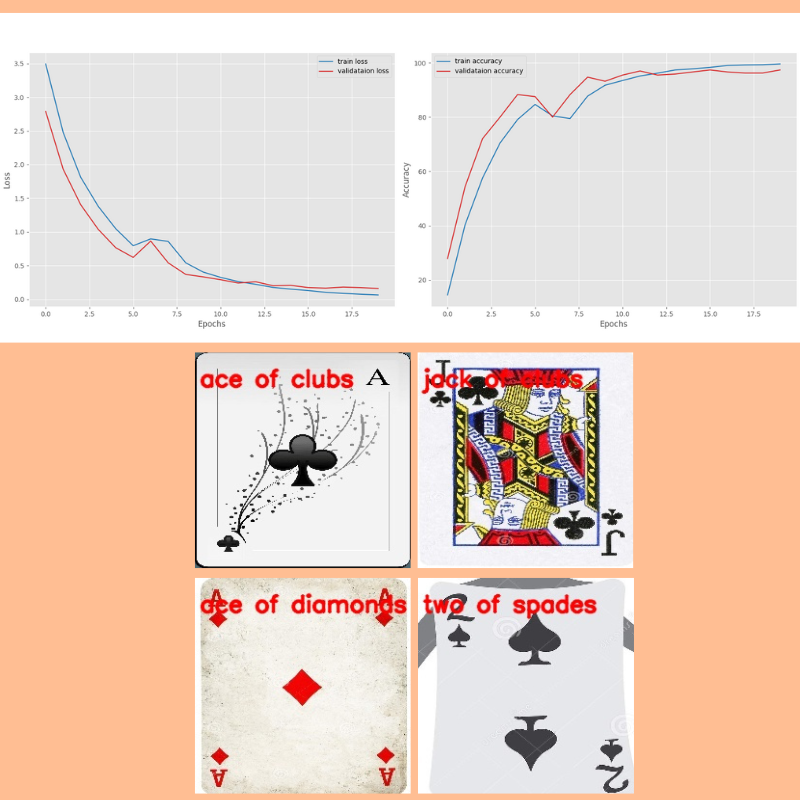
Running Inference on Test Samples
There are a few samples in the input/inference_data folder from the test set. The names represent the class the cards belong to. Let’s run inference using infer_classifier.py script and see how the model performs. We will use the fine-tuned weights from the second experiment.
For inference, we need to load the class names as well. We maintain YAML files for this in the classification_configs directory. For our use case, we have a cards.yaml file with the following content.
CLASS_NAMES: ['ace of clubs', 'ace of diamonds', 'ace of hearts', 'ace of spades',
'eight of clubs', 'eight of diamonds', 'eight of hearts', 'eight of spades',
'five of clubs', 'five of diamonds', 'five of hearts', 'five of spades',
'four of clubs', 'four of diamonds', 'four of hearts', 'four of spades',
'jack of clubs', 'jack of diamonds', 'jack of hearts', 'jack of spades',
'joker', 'king of clubs', 'king of diamonds', 'king of hearts', 'king of spades',
'nine of clubs', 'nine of diamonds', 'nine of hearts', 'nine of spades',
'queen of clubs', 'queen of diamonds', 'queen of hearts', 'queen of spades',
'seven of clubs', 'seven of diamonds', 'seven of hearts', 'seven of spades',
'six of clubs', 'six of diamonds', 'six of hearts', 'six of spades',
'ten of clubs', 'ten of diamonds', 'ten of hearts', 'ten of spades',
'three of clubs', 'three of diamonds', 'three of hearts', 'three of spades',
'two of clubs', 'two of diamonds', 'two of hearts', 'two of spades']
We will pass this as an argument when executing the script.
python infer_classifier.py --weights outputs/fine_tune/best_model.pth --config classification_configs/cards.yaml --model-name dinov3_vits16 --repo-dir dinov3 --input input/inference_data/
We provide the path to the best trained weights, the path to the classification config file, the model name, the repository path, and the directory path containing the images.
Here are the results.

The model was able to classify all the images correctly.
Although this is not extensive testing, we get the idea of the capability of these models.
You can train and test them further on more challenging datasets.
Summary and Conclusion
In this article, we covered how to use DINOv3 for image classification. We started with the discussion of the backbones present and how to load them. Next, we covered how to modify the backbone and add a classifier head on top of it for image classification. Then we trained the model in two different settings and finally carried out inference.
If you have any questions, thoughts, or suggestions, please leave them in the comment section. I will surely address them.
You can contact me using the Contact section. You can also find me on LinkedIn, and X.
References

1 thought on “Image Classification with DINOv3”