JEPA Series Part-3: Image Classification using I-JEPA

In this article, we will use the I-JEPA model for image classification. Using a pretrained I-JEPA model, we will fine-tune it for a downstream image classification task.

In a previous article, we covered the introduction to I-JEPA. If you are new to the I-JEPA series of models, this article will get you up to speed.

This article focuses more on scenarios where we want to tackle a specific image classification task using the learned features of I-JEPA. We will use these models for brain tumor classification.

What are we going to cover in this article?

• Setting up the codebase for image classification using I-JEPA.
• Going over the important code sections and how we integrate the image classification code with a fork of the official I-JEPA repository.
• Training and inference with I-JEPA for image classification.

The Dataset That We Will Use for I-JEPA Image Classification

We will train the I-JEPA model on a brain tumor dataset from here on Kaggle. It contains data for two tasks, image classification and semantic segmentation. However, we will focus on the classification dataset in this article.

We get the following directory structure after downloading and extracting the dataset:

archive
└── brisc2025
    ├── classification_task
    │   ├── test
    │   │   ├── glioma  [254 entries exceeds filelimit, not opening dir]
    │   │   ├── meningioma  [306 entries exceeds filelimit, not opening dir]
    │   │   ├── no_tumor  [140 entries exceeds filelimit, not opening dir]
    │   │   └── pituitary  [300 entries exceeds filelimit, not opening dir]
    │   └── train
    │       ├── glioma  [1147 entries exceeds filelimit, not opening dir]
    │       ├── meningioma  [1329 entries exceeds filelimit, not opening dir]
    │       ├── no_tumor  [1067 entries exceeds filelimit, not opening dir]
    │       └── pituitary  [1457 entries exceeds filelimit, not opening dir]
    └── segmentation_task
        ├── test
        │   ├── images  [860 entries exceeds filelimit, not opening dir]
        │   └── masks  [860 entries exceeds filelimit, not opening dir]
        └── train
            ├── images  [3933 entries exceeds filelimit, not opening dir]
            └── masks  [3933 entries exceeds filelimit, not opening dir]

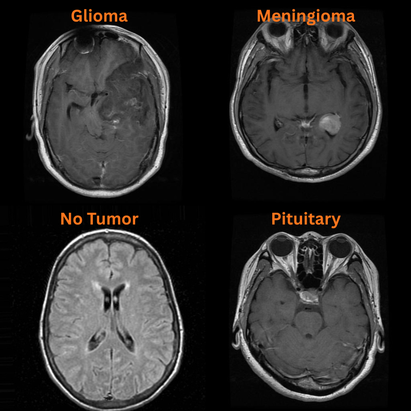
There are two subdirectories, and we will focus on the classification_task one. As we can see, the dataset contains four classes: Glioma, Meningioma, Pituitary Tumor, and No Tumor.

The dataset contains a total of 5000 training and 1000 vlaidation samples.

Following are some of the samples from the dataset.

The I-JEPA Repository

The codebase that we will use here is one that I am maintaining as a fork of the original I-JEPA repository.

This repository additionally contains code for downstream tasks like image classification and semantic segmentation.

As the codebase is prone to significant changes, we will use a stable clone of it in this article, whose zip file will be available for download.

Project Directory Structure

Following is the complete project directory structure.

├── configs
│   ├── in1k_vith14_ep300.yaml
│   ├── in1k_vith16-448_ep300.yaml
│   ├── in22k_vitg16_ep44.yaml
│   └── in22k_vith14_ep66.yaml
├── input
│   ├── archive
│   │   └── brisc2025
│   ├── archive.zip
│   └── readme.txt
├── outputs
├── segmentation_configs
│   ├── person.yaml
│   └── voc.yaml
├── src
│   ├── datasets
│   │   └── imagenet1k.py
│   ├── img_cls
│   │   ├── __pycache__
│   │   ├── datasets.py
│   │   ├── __init__.py
│   │   ├── model.py
│   │   └── utils.py
│   ├── img_seg
│   │   ├── datasets.py
│   │   ├── engine.py
│   │   ├── __init__.py
│   │   ├── metrics.py
│   │   ├── model.py
│   │   └── utils.py
│   ├── masks
│   │   ├── __pycache__
│   │   ├── default.py
│   │   ├── multiblock.py
│   │   ├── random.py
│   │   └── utils.py
│   ├── models
│   │   ├── __pycache__
│   │   └── vision_transformer.py
│   ├── utils
│   │   ├── __pycache__
│   │   ├── distributed.py
│   │   ├── logging.py
│   │   ├── schedulers.py
│   │   └── tensors.py
│   ├── helper.py
│   ├── train.py
│   └── transforms.py
├── weights
│   ├── IN1K-vit.h.14-300e.pth.tar
│   └── readme.txt
├── CODE_OF_CONDUCT.md
├── CONTRIBUTING.md
├── image_similarity_hf.py
├── image_similarity_pt.py
├── infer_classifier.py
├── infer_seg_image.py
├── infer_seg_video.py
├── LICENSE
├── load_model_test.py
├── main_distributed.py
├── main.py
├── NOTES.md
├── README.md
├── requirements.txt
├── train_classifier.py
└── train_segmentation.py

The codebase contains a large number of files, including directories from the original repository. However, we will focus on the following here:

• train_classifier.py and infer_classifier.py scripts for training and inference for image classification, respectively.
• The src/img_cls directory contains all the code related to image classification.
• The dataset that we downloaded above is present in the input directory. All the training and inference results will go into the outputs directory.
• We have all the pretrained weights in the weights directory that we will see later how to download.
• All the major dependencies are listed in the requirements.txt file.

All the fine-tuned weights and code files will be available for download via zip file. If you plan to run training, you will need to download the dataset and arrange it in the above structure. If you wish to just run inference, please download these weights from here and put them in outputs/img_cls directory.

Download Code

Installing Dependencies

We can install all the major dependencies via the requirements file.

pip install -r requirements.txt

This is all the setup we need before diving into the coding section for image classification using I-JEPA.

You can refer to the following article if you want to learn more about how we can use I-JEPA for image similarity.

Code for Image Classification Using I-JEPA

In this section, we will cover some of the important code files and their usage in the codebase. However, as it can be quite lengthy, we will not go through the code of each file; rather will describe what it does.

Downloading the Pretrained Weights

We will fine-tune the ViT-Huge model trained with 14×14 patches pretrained on the ImageNet1K dataset. All the pretrained weights are available here. You can click on this link to download the particular model. After downloading, this goes into the weights directory.

Code for Model Preparation

The code to initialize the model for image classification and load the pretrained weights is present in the src/img_cls/models.py file.

We use a simple linear layer classifier on top of the frozen features.

class LinearClassifier(nn.Module):
    def __init__(self, num_classes=10, fine_tune=False, weights=None):
        super(LinearClassifier, self).__init__()

        if weights is not None:
            backbone_model = load_model(weights=weights)
        else:
            backbone_model = vit_huge(patch_size=14)

        self.model = torch.nn.Sequential(OrderedDict([
            ('backbone', backbone_model),
            ('head', torch.nn.Linear(
                in_features=1280, out_features=num_classes, bias=True
            ))
        ]))
    
        if not fine_tune:
            for params in self.model.backbone.parameters():
                params.requires_grad = False

    def forward(self, x):
        backbone_out = self.model.backbone(x)
        avg_features = backbone_out.mean(dim=1)
        out = self.model.head(avg_features)

        return out

We take the mean of the features from the pretrained backbone. This gives us features with shape [batch_size, embedding_dim] that we feed into the linear layer. The embedding dimension for the model that we are using is 1280, so our Linear layer has an input feature size of 1280.

Code for Dataset Preparation

All the dataset preparation code is present in the src/img_cls/datasets.py file. It contains all the dataset transforms for training and validation data preparation, creates the PyTorch datasets and data loaders, and finally returns them to the main script.

We are resizing all the images to 256×256 resolution and center cropping them to 224×224 resolution. Additionally, we apply horizontal flipping augmentations to the training samples with a probability of 0.5.

Code for Utilities and Helper Functions

The utilities and helper functions are present in the src/img_cls/utils.py file. This contains the following:

• Class to save the best model weights according to the least validation loss.
• Function to save the last model.
• Function to save the accuracy and loss plots.

The Main Training Script

The train_classifier.py in the root directory is the executable script that starts the training process. It imports all the necessary modules, prepares and loads the model, and initializes the data loaders as well. It also contains the logic for training and validation loops.

Furthermore, we have the following command line arguments that we can pass to the script.

# Construct the argument parser.
parser = argparse.ArgumentParser()
parser.add_argument(
    '-e', '--epochs', 
    type=int, 
    default=10,
    help='Number of epochs to train our network for'
)
parser.add_argument(
    '-lr', '--learning-rate', 
    type=float,
    dest='learning_rate', 
    default=0.001,
    help='Learning rate for training the model'
)
parser.add_argument(
    '-b', '--batch-size',
    dest='batch_size',
    default=32,
    type=int
)
parser.add_argument(
    '--save-name',
    dest='save_name',
    default='model',
    help='file name of the final model to save'
)
parser.add_argument(
    '--fine-tune',
    dest='fine_tune',
    action='store_true',
    help='whether to fine-tune the model or train the classifier layer only'
)
parser.add_argument(
    '--out-dir',
    dest='out_dir',
    default='img_cls',
    help='output sub-directory path inside the `outputs` directory'
)
parser.add_argument(
    '--scheduler',
    type=int,
    nargs='+',
    default=[1000],
    help='number of epochs after which learning rate scheduler is applied'
)
parser.add_argument(
    '--train-dir',
    dest='train_dir',
    required=True,
    help='path to the training directory containing class folders in \
          PyTorch ImageFolder format'
)
parser.add_argument(
    '--valid-dir',
    dest='valid_dir',
    required=True,
    help='path to the validation directory containing class folders in \
          PyTorch ImageFolder format'
)
args = parser.parse_args()

All of them are pretty much self-explanatory.

The --train-dir and --valid-dir arguments accept directory paths that contain the dataset samples in PyTorch ImageFolder format. The --out-dir is the subdirectory path inside the outputs directory that will be created for saving the results.

Training the I-JEPA Model for Image Classification

All the training and inference experiments were done on a machine with 10GB RTX 3080 GPU, 32GB RAM, and an i7 10th-generation processor.

Let’s execute the training script.

python train_classifier.py --train-dir input/archive/brisc2025/classification_task/train/ --valid-dir input/archive/brisc2025/classification_task/test/ --learning-rate 0.001 --out-dir img_cls

We are training for the default number of epochs, that is 10, with a learning rate of 0.001 without any scheduling. Following is the truncated output from the terminal.

Namespace(epochs=10, learning_rate=0.001, batch_size=32, save_name='model', fine_tune=False, out_dir='trial', scheduler=[1000], train_dir='data/archive/brisc2025/classification_task/train/', valid_dir='data/archive/brisc2025/classification_task/test/')
[INFO]: Number of training images: 5000
[INFO]: Number of validation images: 1000
[INFO]: Classes: ['glioma', 'meningioma', 'no_tumor', 'pituitary']
Computation device: cuda
Learning rate: 0.001
Epochs to train for: 10

dict_keys(['encoder', 'predictor', 'opt', 'scaler', 'target_encoder', 'epoch', 'loss', 'batch_size', 'world_size', 'lr'])
############################## Model ##############################
VisionTransformer(
  (patch_embed): PatchEmbed(
    (proj): Conv2d(3, 1280, kernel_size=(14, 14), stride=(14, 14))
  )
  (blocks): ModuleList(
    (0-31): 32 x Block(
      (norm1): LayerNorm((1280,), eps=1e-06, elementwise_affine=True)
      (attn): Attention(
        (qkv): Linear(in_features=1280, out_features=3840, bias=True)
        (attn_drop): Dropout(p=0.0, inplace=False)
        (proj): Linear(in_features=1280, out_features=1280, bias=True)
        (proj_drop): Dropout(p=0.0, inplace=False)
      )
      (drop_path): Identity()
      (norm2): LayerNorm((1280,), eps=1e-06, elementwise_affine=True)
      (mlp): MLP(
        (fc1): Linear(in_features=1280, out_features=5120, bias=True)
        (act): GELU(approximate='none')
        (fc2): Linear(in_features=5120, out_features=1280, bias=True)
        (drop): Dropout(p=0.0, inplace=False)
      )
    )
  )
  (norm): LayerNorm((1280,), eps=1e-06, elementwise_affine=True)
)
###################################################################
.
.
.
630,767,364 total parameters.
5,124 training parameters.
[INFO]: Epoch 1 of 10
Training
100%|██████████████████████████████████████████████████████████████████████████████████████████████████████████████████████████████████████████████████████| 157/157 [02:06<00:00,  1.24it/s]
Validation
100%|████████████████████████████████████████████████████████████████████████████████████████████████████████████████████████████████████████████████████████| 32/32 [00:25<00:00,  1.24it/s]
Training loss: 0.793, training acc: 73.400
Validation loss: 0.737, validation acc: 72.000

Best validation loss: 0.7367627648636699

Saving best model for epoch: 1

--------------------------------------------------
.
.
.
LR for next epoch: [0.001]
[INFO]: Epoch 9 of 10
Training
100%|██████████████████████████████████████████████████████████████████████████████████████████████████████████████████████████████████████████████████████| 157/157 [02:04<00:00,  1.26it/s]
Validation
100%|████████████████████████████████████████████████████████████████████████████████████████████████████████████████████████████████████████████████████████| 32/32 [00:24<00:00,  1.28it/s]
Training loss: 0.305, training acc: 89.920
Validation loss: 0.414, validation acc: 82.600

Best validation loss: 0.413845632574521

Saving best model for epoch: 9

--------------------------------------------------
LR for next epoch: [0.001]
[INFO]: Epoch 10 of 10
Training
100%|██████████████████████████████████████████████████████████████████████████████████████████████████████████████████████████████████████████████████████| 157/157 [01:51<00:00,  1.41it/s]
Validation
100%|████████████████████████████████████████████████████████████████████████████████████████████████████████████████████████████████████████████████████████| 32/32 [00:22<00:00,  1.44it/s]
Training loss: 0.296, training acc: 90.380
Validation loss: 0.419, validation acc: 82.300
--------------------------------------------------
LR for next epoch: [0.001]
TRAINING COMPLETE

As the backbone is frozen, the entire model has only 5124 trainable parameters.

The best model, according to the least validation loss, was saved on epoch 9. The model reached the best validation accuracy of 82.6% on the same epoch.

Here are the accuracy and loss plots.

We could have trained for a bit longer to check whether there were improvements or whether learning rate scheduling would be needed for further training.

Inference Using the Trained I-JEPA Model for Image Classification

The code for running inference using the trained image classification model is present in the infer_classifier.py file. Following is the entire code.

"""
Script for image classification inference using trained model.

USAGE:
python infer_classifier.py --weights <path to the weights.pth file> \
--input <directory containing inference images>

Update the `CLASS_NAMES` list to contain the trained class names. 
"""

import torch
import numpy as np
import cv2
import os
import torch.nn.functional as F
import torchvision.transforms as transforms
import glob
import argparse
import pathlib

from src.img_cls.model import LinearClassifier

# Construct the argument parser.
parser = argparse.ArgumentParser()
parser.add_argument(
    '-w', '--weights', 
    default='../outputs/best_model.pth',
    help='path to the model weights',
)
parser.add_argument(
    '--input',
    required=True,
    help='directory containing images for inference'
)
args = parser.parse_args()

# Constants and other configurations.
DEVICE = torch.device('cuda:0' if torch.cuda.is_available() else 'cpu')
IMAGE_RESIZE = 256
CLASS_NAMES = ['glioma', 'meningioma', 'no_tumor', 'pituitary']

# Validation transforms
def get_test_transform(image_size):
    test_transform = transforms.Compose([
        transforms.ToPILImage(),
        transforms.Resize((image_size, image_size)),
        transforms.CenterCrop((224, 224)),
        transforms.ToTensor(),
        transforms.Normalize(
            mean=(0.485, 0.456, 0.406),
            std=(0.229, 0.224, 0.225)
        )
    ])
    return test_transform

def annotate_image(output_class, orig_image):
    class_name = CLASS_NAMES[int(output_class)]
    cv2.putText(
        orig_image, 
        f"{class_name}", 
        (5, 35), 
        cv2.FONT_HERSHEY_SIMPLEX, 
        0.8, 
        (0, 0, 255), 
        2, 
        lineType=cv2.LINE_AA
    )
    return orig_image

def inference(model, testloader, device, orig_image):
    """
    Function to run inference.

    :param model: The trained model.
    :param testloader: The test data loader.
    :param DEVICE: The computation device.
    """
    model.eval()
    counter = 0

    with torch.no_grad():
        counter += 1
        image = testloader
        image = image.to(device)

        # Forward pass.
        outputs = model(image)

    # Softmax probabilities.
    predictions = F.softmax(outputs, dim=1).cpu().numpy()
    # Predicted class number.
    output_class = np.argmax(predictions)
    # Show and save the results.
    result = annotate_image(output_class, orig_image)
    return result

if __name__ == '__main__':
    weights_path = pathlib.Path(args.weights)
    infer_result_path = os.path.join(
        'outputs', 'inference_results'
    )
    os.makedirs(infer_result_path, exist_ok=True)

    checkpoint = torch.load(weights_path)
    # Load the model.
    model = LinearClassifier(
        num_classes=len(CLASS_NAMES)
    ).to(DEVICE)
    model.load_state_dict(checkpoint['model_state_dict'])

    all_image_paths = glob.glob(os.path.join(args.input, '*'))

    transform = get_test_transform(IMAGE_RESIZE)

    for i, image_path in enumerate(all_image_paths):
        print(f"Inference on image: {i+1}")
        image = cv2.imread(image_path)
        orig_image = image.copy()
        image = cv2.cvtColor(image, cv2.COLOR_BGR2RGB)
        image = transform(image)
        image = torch.unsqueeze(image, 0)
        result = inference(
            model, 
            image,
            DEVICE,
            orig_image
        )
        # Save the image to disk.
        image_name = image_path.split(os.path.sep)[-1]
        # cv2.imshow('Image', result)
        # cv2.waitKey(1)
        cv2.imwrite(
            os.path.join(infer_result_path, image_name), result
        )

Currently, one of the downsides of the script is that we need to modify the CLASS_NAMES list for each dataset we are dealing with. For our current use case, we have updated the class names to match those present in the dataset.

There are four images in the input/inference_data directory representing one image from each class. The file names represent the ground truth class.

inference_data/
├── glioma.jpg
├── meningioma.jpg
├── no_tumor.jpg
└── pituitary.jpg

Let’s run inference and analyze how our trained model performs.

python infer_classifier.py --weights outputs/img_cls/best_model.pth --input input/inference_data/

After the inference is complete, the results are stored in outputs/inference_results directory.

The following are the results. The red text represents the predictions and the green text the ground truth labels.

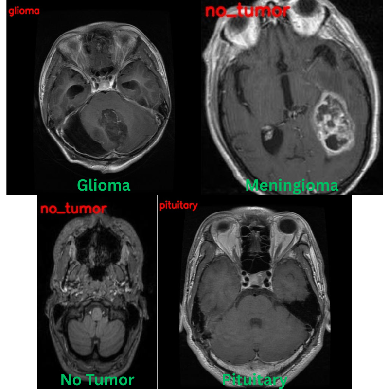
Apart from one image, that is meningioma predicted as no_tumor, the other three predictions are correct.

During training, calculating the class-wise classification accuracy scores and using learning rate scheduling with longer training will surely improve the results.

Summary and Conclusion

In this article, we covered image classification using I-JEPA. Using the strong pretrained features of I-JEPA, we added a simple classifier head on top of the backbone and trained the model for brain tumor classification. Along the way, we discussed how the code files are structured and what kind of results we can expect upon further improvements.

If you have any questions, thoughts, or suggestions, please leave them in the comment section. I will surely address them.

You can contact me using the Contact section. You can also find me on LinkedIn, and X.