Hyperparameter Search with PyTorch and Skorch

In this tutorial, we will carry out hyperparameter search (and then tuning) using the PyTorch deep learning framework along with Skorch.

In the last two tutorials, we covered the following points:

• The theoretical aspects of hyperparameter search and tuning in deep learning.
• Manual hyperparameter tuning in deep learning in PyTorch.

By now, we have a good idea of how difficult it is to search for good hyperparameters in deep learning. Also, as we saw in the previous post, manual hyperparameter tuning in deep learning is not a very good idea either.

That brings us to this tutorial today. We will try to automate a few aspects of hyperparameter search for a deep learning model built with PyTorch. And for that, we will use the Skorch library.

Let’s take a look at the points that we will cover in this post.

• We will start with building a neural network model using PyTorch.
• We will then move on to defining and preparing the datasets.
• Moving ahead, we will write a simple script for hyperparameter search using PyTorch and Skorch. Specifically, we will carry out Grid Search of the hyperparameters.
• After we obtain the best hyperparameters, we will use those to train a final model.
• The dataset in this tutorial is same as the previous one. So, we will be able to compare whether our extra effort of hyperparameter search was beneficial or not.
• We will end the post with some of the pros and cons of using Grid Search for searching the best hyperparameters for neural network training.

Note: More than 90% of the code in this post will be similar to the previous one. For that reason, we may not go into an in-depth explanation of each part. Whichever part is new, we will surely dive into those explanations (code for Skorch in particular). If you are directly visiting this post, I highly recommend at least skimming through the previous post just to get an idea of the code. Also, the dataset will be the same as the previous post so that we can compare the results in the end.

Let’s begin.

The Dataset

As already discussed above, we will be using the same Natural Images from Kaggle in this post. To get to know the dataset well, you may visit this link or the previous post. Still, just reiterating the important points here:

• It has 8 classes: airplane, car, cat, dog, flower, fruit, motorbike, person.
• And a total of 6899 images.

You can download the dataset from here. In the next section, we will explore how to structure the project folder along with the dataset directory.

The Directory Structure

The following block shows the directory structure for the project.

├── input
│   └── natural_images
│       ├── airplane [727 entries exceeds filelimit, not opening dir]
│       ├── car [968 entries exceeds filelimit, not opening dir]
│       ├── cat [885 entries exceeds filelimit, not opening dir]
│       ├── dog [702 entries exceeds filelimit, not opening dir]
│       ├── flower [843 entries exceeds filelimit, not opening dir]
│       ├── fruit [1000 entries exceeds filelimit, not opening dir]
│       ├── motorbike [788 entries exceeds filelimit, not opening dir]
│       └── person [986 entries exceeds filelimit, not opening dir]
├── outputs
│   ├── run_1
│   │   ├── accuracy.png
│   │   ├── hyperparam.yml
│   │   └── loss.png
│   └── search_1
│       └── best_param.yml
└── src
    ├── datasets.py
    ├── model.py
    ├── search.py
    ├── train.py
    └── utils.py

• The input folder contains the natural_images data folder which contains the images inside the respective class directories.
• The outputs directory will cotnain the outputs of the hyperparameter search and training results as well. We will get into the details of these while writing the code to create these directories.
• Inside the src directory we have the 5 Python files that we will be dealing with and writing code for in this tutorial.

As you can see this project, that is, hyperparameter search with PyTorch and Skorch has only one additional Python script, search.py.

Downloading the zip file for this tutorial will already provide you with everything with the above directory structure. You just need to download the dataset and extract it inside the input folder.

Libraries and Dependencies

There are three major libraries that we will need in this tutorial. They are:

• PyTorch (the deep learning framwork of choice for this tutorial):
  • If you don’t yet have it on your system, you can install it by visiting the official site here.
• Skorch:
  • You will also need Skorch and you can install it according to your requirements from here.
• Scikit-Learn:
  • We will be using the Grid Search module from Scikit-Learn. Install it from here depending on your system.

A Bit About Skorch

We know that PyTorch is a great deep learning framework. But it does not support hyperparameter search and tuning natively. That’s where Skorch comes in. So, what is Skorch?

Quoting a few lines from the Skorch documentation here.

A scikit-learn compatible neural network library that wraps PyTorch.
The goal of skorch is to make it possible to use PyTorch with sklearn. This is achieved by providing a wrapper around PyTorch that has an sklearn interface.

Skorch docs

The above few lines iterate the functionality of Skorch quite well. In even simpler terms, to access the modules and functionalities of Scikit-Learn and use them with PyTorch, Skorch will act as a medium. And one such requirement is the Grid Search module of Sciki-Learn that we are going to use in this tutorial. All in all, to apply Grid Search to hyperparameters of a neural network, we also need the Scikit-Learn library along with Skorch.

But the usefulness of Skorch does not end here. There are many others and it’s fascinating how it entangles everything with Scikit-Learn like code. Do visit the docs to know more. In fact, we may just explore a few of these in future tutorials.

For now, let’s move on to the coding part of the tutorial.

Hyperparameter Search with PyTorch and Skorch

Note: Most of the code will remain the same as in the previous post. One additional script that we have here is the search.py which carries out the hyperparameter search. There are some caveats to blindly executing this script which we will learn about after writing its code and before executing it.

We will cover the code files in the following order:

• utils.py
• datasets.py
• model.py
• search.py
• train.py

The Utilities Script

We will write some helper functions in the utils.py file. There are a total of 5 functions in the file, out of which the first three are the same as the previous post.

import matplotlib
import matplotlib.pyplot as plt
import glob as glob
import os

matplotlib.style.use('ggplot')

def save_plots(
    train_acc, valid_acc, train_loss, valid_loss, 
    acc_plot_path, loss_plot_path
):
    """
    Function to save the loss and accuracy plots to disk.
    """
    # Accuracy plots.
    plt.figure(figsize=(10, 7))
    plt.plot(
        train_acc, color='green', linestyle='-', 
        label='train accuracy'
    )
    plt.plot(
        valid_acc, color='blue', linestyle='-', 
        label='validataion accuracy'
    )
    plt.xlabel('Epochs')
    plt.ylabel('Accuracy')
    plt.legend()
    plt.savefig(acc_plot_path)
    
    # Loss plots.
    plt.figure(figsize=(10, 7))
    plt.plot(
        train_loss, color='orange', linestyle='-', 
        label='train loss'
    )
    plt.plot(
        valid_loss, color='red', linestyle='-', 
        label='validataion loss'
    )
    plt.xlabel('Epochs')
    plt.ylabel('Loss')
    plt.legend()
    plt.savefig(loss_plot_path)

def save_hyperparam(text, path):
    """
    Function to save hyperparameters in a `.yml` file.

    :param text: The hyperparameters dictionary.
    :param path: Path to save the hyperparmeters.
    """
    with open(path, 'w') as f:
        keys = list(text.keys())
        for key in keys:
            f.writelines(f"{key}: {text[key]}\n")

def create_run():
    """
    Function to create `run_<num>` folders in the `outputs` folder for each run.
    """
    num_run_dirs = len(glob.glob('../outputs/run_*'))
    run_dir = f"../outputs/run_{num_run_dirs+1}"
    os.makedirs(run_dir)
    return run_dir 

We just have a minor change in the create_run() function for defining the run_dir variable (line 62), no other changes.

In addition to this, we have two more functions.

def creat_search_run():
    """
    Function to save the Grid Search results.
    """
    num_search_dirs = len(glob.glob('../outputs/search_*'))
    search_dirs = f"../outputs/search_{num_search_dirs+1}"
    os.makedirs(search_dirs)
    return search_dirs

def save_best_hyperparam(text, path):
    """
    Function to save best hyperparameters in a `.yml` file.


    :param text: The hyperparameters dictionary.
    :param path: Path to save the hyperparmeters.
    """
    with open(path, 'a') as f:
        f.write(f"{str(text)}\n")

• The create_search_run() function creates another set of folder inside the outputs directory. The naming format is search_<dir_number>. This will be created everytime we execute the search.py script so that the best hyperparameters of the search can be saved to a new folder without overwriting the previous one.
• The save_best_hyperparam() will create a .yml file for the current search run inside the search_<dir_number> directory and save the best hyperaparameter of search along with the best accuracy score. You might get an even better idea by looking at the directory structure in the above section to check how the directories are named.

So, we don’t need to create a new directory for each search run or train run. These helper functions will take care of this for us.

Preparing the Dataset

The dataset preparation code will go into the datasets.py file and is exactly the same as we had in the previous post.

To keep the tutorial streamlined and easy to follow, I am including the entire code for dataset preparation in the following code block.

import torch

from torch.utils.data import DataLoader, Subset
from torchvision import datasets, transforms

# Ratio of split to use for validation.
VALID_SPLIT = 0.1
# Batch size.
BATCH_SIZE = 64
# Path to data root directory.
ROOT_DIR = '../input/natural_images'

# Training transforms
def get_train_transform(IMAGE_SIZE):
    train_transform = transforms.Compose([
        transforms.Resize((IMAGE_SIZE, IMAGE_SIZE)),
        transforms.ToTensor(),
        transforms.Normalize(
            mean=[0.5, 0.5, 0.5],
            std=[0.5, 0.5, 0.5]
        )
    ])
    return train_transform


# Validation transforms
def get_valid_transform(IMAGE_SIZE):
    valid_transform = transforms.Compose([
        transforms.Resize((IMAGE_SIZE, IMAGE_SIZE)),
        transforms.ToTensor(),
        transforms.Normalize(
            mean=[0.5, 0.5, 0.5],
            std=[0.5, 0.5, 0.5]
        )
    ])
    return valid_transform


# Initial entire datasets,
# same for the entire and test dataset.
def get_datasets(IMAGE_SIZE):
    dataset = datasets.ImageFolder(ROOT_DIR, transform=get_train_transform(IMAGE_SIZE))
    dataset_test = datasets.ImageFolder(ROOT_DIR, transform=get_valid_transform(IMAGE_SIZE))
    print(f"Classes: {dataset.classes}")
    dataset_size = len(dataset)
    print(f"Total number of images: {dataset_size}")

    valid_size = int(VALID_SPLIT*dataset_size)

    # Training and validation sets
    indices = torch.randperm(len(dataset)).tolist()
    dataset_train = Subset(dataset, indices[:-valid_size])
    dataset_valid = Subset(dataset_test, indices[-valid_size:])

    print(f"Total training images: {len(dataset_train)}")
    print(f"Total valid_images: {len(dataset_valid)}")
    return dataset_train, dataset_valid, dataset.classes


# Training and validation data loaders.
def get_data_loaders(IMAGE_SIZE):
    dataset_train, dataset_valid, dataset_classes = get_datasets(IMAGE_SIZE)
    train_loader = DataLoader(
        dataset_train, batch_size=BATCH_SIZE, shuffle=True, num_workers=4
    )
    valid_loader = DataLoader(
        dataset_valid, batch_size=BATCH_SIZE, shuffle=False, num_workers=4
    )
    return train_loader, valid_loader, dataset_classes 

• We use 10% of the data for validation with a batch size of 64.
• We do not use any image augmentation techniques here. Both, training and validation transforms following the same set of transforms. This will help us compare the results to the previous post later on.

The Neural Network Model

The same goes for the neural network model as well.

We have a CustomNet() class that we used in the last post. This code will go into the model.py file.

import torch.nn as nn
import torch.nn.functional as F
import torch

class CustomNet(nn.Module):
    def __init__(self, first_conv_out, first_fc_out):
        super().__init__()

        self.first_conv_out = first_conv_out
        self.first_fc_out = first_fc_out

        # All Conv layers.
        self.conv1 = nn.Conv2d(3, self.first_conv_out, 5)
        self.conv2 = nn.Conv2d(self.first_conv_out, self.first_conv_out*2, 3)
        self.conv3 = nn.Conv2d(self.first_conv_out*2, self.first_conv_out*4, 3)
        self.conv4 = nn.Conv2d(self.first_conv_out*4, self.first_conv_out*8, 3)
        self.conv5 = nn.Conv2d(self.first_conv_out*8, self.first_conv_out*16, 3)

        # All fully connected layers.
        self.fc1 = nn.Linear(self.first_conv_out*16, self.first_fc_out)
        self.fc2 = nn.Linear(self.first_fc_out, self.first_fc_out//2)
        self.fc3 = nn.Linear(self.first_fc_out//2, 8)

        # Max pooling layers
        self.pool = nn.MaxPool2d(2, 2)

    def forward(self, x):    
        # Passing though convolutions.
        x = self.pool(F.relu(self.conv1(x)))
        x = self.pool(F.relu(self.conv2(x)))
        x = self.pool(F.relu(self.conv3(x)))
        x = self.pool(F.relu(self.conv4(x)))
        x = self.pool(F.relu(self.conv5(x)))

        # Flatten.
        bs, _, _, _ = x.shape
        x = F.adaptive_avg_pool2d(x, 1).reshape(bs, -1)
        x = F.relu(self.fc1(x))
        x = F.relu(self.fc2(x))
        x = self.fc3(x)
        return x

if __name__ == '__main__':
    model = CustomNet()
    tensor = torch.randn(1, 3, 224, 224)
    output = model(tensor)
    print(output.shape)

Basically, we treat the output channels of the first convolutional layer and output features of the first fully connected layer as hyperparameters. As you can see from the code, the rest of the neural network gets built according to these two inputs.

The Hyperparameter Search Code

This is an important part of the tutorial and entirely new as well. Here, we will write the code for hyperparameter search using the Grid Search method from Scikit-Learn and using the Skorch library modules as a wrapper around the neural network model.

Things might sound complicated as of now. But let’s write the code first. It will become much simpler.

This code will go into the search.py script.

First, let’s deal with all the import statements.

import torch
import torch.nn as nn

from skorch import NeuralNetClassifier
from sklearn.model_selection import GridSearchCV

from utils import creat_search_run, save_best_hyperparam
from model import CustomNet
from datasets import get_data_loaders

We can see a few new imports in the above code block.

• The NeuralNetClassifier class from skorch which will be wrapper around our own neural network model.
• And the GridSearchCV class from sklearn to carry out the hyperparameter search.

Along with that, we also import our own classes and function from the utils, model, and datasets modules.

The Main Code Block for Hyperparameter Search

The entire main code for hyperparameter search using PyTorch and Skorch is contained within the next code block. Let’s write the code first, then move over to the explanation.

if __name__ == '__main__':
    # Create hyperparam search folder.
    search_folder = creat_search_run()

    # Learning parameters. 
    lr = 0.001
    epochs = 20
    device = 'cpu'
    print(f"Computation device: {device}\n")

    # Loss function. Required for defining `NeuralNetClassifier`
    criterion = nn.CrossEntropyLoss()

    
    # Instance of `NeuralNetClassifier` to be passed to `GridSearchCV` 
    net = NeuralNetClassifier(
        module=CustomNet, max_epochs=epochs,
        optimizer=torch.optim.Adam,
        criterion=criterion,
        lr=lr, verbose=1
    )

    # Get the training and validation data loaders.
    train_loader, valid_loader, dataset_classes = get_data_loaders(224)

    
    params = {
    'lr': [0.001, 0.01, 0.005, 0.0005],
    'max_epochs': list(range(20, 55, 5)),
    'module__first_conv_out': [4, 8, 16, 32],
    'module__first_fc_out': [128, 256, 512],
    }

    """
    Define `GridSearchCV`.
    4 lrs * 7 max_epochs * 4 module__first_conv_out * 3 module__first_fc_out
    * 2 CVs = 672 fits.
    """
    gs = GridSearchCV(
        net, params, refit=False, scoring='accuracy', verbose=1, cv=2
    )

    counter = 0
    # Run each fit for 2 batches. So, if we have `n` fits, then it will
    # actually for `n*2` times. We have 672 fits, so total, 
    # 672 * 2 = 1344 runs.
    search_batches = 2
    """
    This will run `n` (`n` is calculated from `params`) number of fits 
    on each batch of data, so be careful.
    If you want to run the `n` number of fits just once, 
    that is, on one batch of data,
    add `break` after this line:
        `outputs = gs.fit(image, labels)`

    Note: This will take a lot of time to run
    """
    for i, data in enumerate(train_loader):
        counter += 1
        image, labels = data
        image = image.to(device)
        labels = labels.to(device)
        outputs = gs.fit(image, labels)
        # GridSearch for `search_batches` number of times.
        if counter == search_batches:
            break

    print('SEARCH COMPLETE')
    print("best score: {:.3f}, best params: {}".format(gs.best_score_, gs.best_params_))
    save_best_hyperparam(gs.best_score_, f"../outputs/{search_folder}/best_param.yml")
    save_best_hyperparam(gs.best_params_, f"../outputs/{search_folder}/best_param.yml")

The very first thing we do is create the search folder inside the outputs directory to save the best hyperparameters.

After that, we define the learning parameters, which are the learning rate and the epochs. We also define the computation device, which is the CPU in this case. Although we are using PyTorch for building the neural network model, the hyperparameter search will happen through the GridSearchCV class of Scikit-Learn. Because of that, we cannot use GPU as the computation device. Although possible it is not very straightforward to use GPU for Grid Search with Skorch + PyTorch yet.

Next, we define the loss function by initializing the criterion variable on line 21.

Starting from line 25, we initialize the NeuralNetClassifier class. Let’s take a look at the arguments that we are passing:

• module: This takes the neural network class, which is CustomNet in our case.
• max_epochs: The number of epochs.
• optimizer: The PyTorch optimizer, which is Adam in this case.
• criterion: The loss function.
• lr: The learning rate.

The above provides us with NeuralNetClassifier instance as net. Now note that arguments that we passed here are the ones generally passed if we would have used net.fit later on for training. But we will be performing Grid Search here. So, things will change a bit further on.

On line 33, we get the data loaders which is quite straightforward.

The Hyperparameters to Search for

Line 36 contains the important bit, which is the params dictionary for the hyperparameter search. The keys are just not keys, but also keywords to be treated as arguments for hyperparameter search by Skorch.

• lr: A list containing all the learning rates we want to search through. A total of four values here.
• max_epochs: The maximum number of epochs to train for. In our case, we start with 20 epoch, slowly move up to 50 epochs with a step size of 5. Total, 7 values.
• module__first_conv_out: This is important. Now you might remember, the neural network initialization requires a first_conv_out argument defining the number of output channels for the first convolutional layer. Here, module__ indicates that the keyword following it, that is, first_conv_out is one of the parameters of the module argument of the net instance that we created above. So, this will also act as a hyperparameter to search for. We search for the best value from [4, 8, 16, 32], 4 values in total.
• module__first_fc_out: This is similar to above, but for the first_fc_out argument of the neural network. Again we search from [128, 256, 512], totalling 3 values.

In total, we have 4 * 7 * 4 * 3 = 336 grids to search as of now. They are a lot. But we are not done yet.

On line 48, we initialize GridSearchCV by passing net and params as arguments. The scoring criterion is accuracy and we carry out 2 cross-validations (cv) for each grid search.

This brings us to our next calculation, that is, 336 grid search * 2 CVs for each = 672 fits in total. Now that’s a lot.

So, the algorithm will run the data through the network 672 times. But there is still more, which is kind of optional.

We Cannot Fit the Entire Dataset in Memory

Obviously, we cannot fit the entire dataset in memory. So, we just do as we do during training, that is, fitting on one batch at a time.

Now, we need to keep in mind that each of the 672 fits will run over one batch. So, iterating over one batch, running, gs.fit(image, labels), and breaking out of the loop would mean running all the 672 fits. Meaning, running all the batches (say 20, for example), would make a total of 13440 fits. And that would take a lot of time (maybe a day on a modest CPU). Remember that we are running the search on a CPU here.

So, what to do?

We initialize a search_batches variable with 2 in our case. So, whenever the batch counter reaches 2, it will break out of the loop. This means that we run for 1344 fits, which is still a lot to be fair. And you need to be careful here while running this as it might take a lot of time to complete.

Finally, we print the best Grid Search score and the best hyperparameters found. We also save them to the .yml file, so that we don’t lose them.

That’s it. The above sums up all the computational things we need to take care of while carrying out Grid Search. Just one more thing. We could have used the n_jobs argument when initializing GridSearchCV indicating the number of parallel processes to use. Now that entirely depends on an individual’s machine. By default it’s 1, make it -1 to use all the cores’ threads. Or give a suitable amount according to your processor.

Running search.py for Hyperparameter Search with PyTorch and Skorch

On a system with i7 10700K and n_jobs=1 (as with the current code in this tutorial), it took around 3 hours to complete the search. If you have a better system or allow more processes, it will be faster. If you are skeptical that it might take long, then you are free to skip it as well and just observe through this section.

Enter the src directory, open up your command line/terminal, and execute the following command.

python search.py

By the end of the execution, you should see an output similar to the following.

/home/sovit/miniconda3/envs/torch110/lib/python3.9/site-packages/sklearn/model_selection/_split.py:676: UserWarning: The least populated class in y has only 2 members, which is less than n_splits=5.
  warnings.warn(
  epoch    train_loss    valid_acc    valid_loss     dur
-------  ------------  -----------  ------------  ------
      1        2.0845       0.1429        2.0751  0.5739
      2        2.0780       0.1429        2.0755  0.5719
      3        2.0698       0.1429        2.0774  0.5735
      4        2.0548       0.1429        2.0886  0.5754
      5        2.0280       0.1429        2.1523  0.5742
      6        1.9980       0.1429        2.3048  0.5740
      7        1.9973       0.1429        2.2622  0.5757
      8        1.9615       0.1429        2.2151  0.5740
      9        1.9410       0.1429        2.2132  0.5747
     10        1.9174       0.1429        2.2641  0.5768
     11        1.8793       0.1429        2.3797  0.5739
     12        1.8398       0.1429        2.4099  0.5700
     13        1.7876       0.1429        2.3575  0.5671
     14        1.7372       0.1429        2.4667  0.5745
     15        1.6892       0.1429        2.7904  0.5645
     16        1.6467       0.1429        2.6569  0.5716
     17        1.5875       0.1429        2.9143  0.5723
     18        1.5207       0.2857        3.3248  0.5734
     19        1.4631       0.1429        3.2598  0.5712
     20        1.4741       0.2857        4.5757  0.5756
     21        1.5312       0.1429        3.4627  0.5764
     22        1.3534       0.1429        3.0494  0.5809
     23        1.4220       0.1429        3.2345  0.5820
     24        1.2990       0.2857        3.9088  0.5793
     25        1.3459       0.2857        3.5109  0.5713
     26        1.2593       0.1429        2.9436  0.5765
     27        1.2467       0.1429        2.9393  0.5773
     28        1.2217       0.4286        3.4453  0.5763
     29        1.1478       0.2857        3.7686  0.5768
     30        1.1471       0.5714        3.1646  0.5774
     31        1.0701       0.2857        3.1794  0.5837
     32        1.0508       0.4286        4.0320  0.5761
     33        1.0246       0.4286        3.8586  0.5807
     34        0.9456       0.2857        3.6610  0.5691
     35        0.9803       0.4286        4.8985  0.5677
     36        0.9300       0.2857        4.5390  0.5756
     37        0.8522       0.2857        4.3094  0.5785
     38        0.8635       0.5714        5.7643  0.5789
     39        0.8707       0.4286        4.9866  0.5761
     40        0.7692       0.4286        5.0372  0.5770
     41        0.7429       0.5714        5.9976  0.5737
     42        0.7522       0.4286        5.5152  0.5774
     43        0.6562       0.4286        5.7557  0.5762
     44        0.6523       0.5714        6.8458  0.5762
     45        0.6368       0.4286        6.5533  0.5775
     46        0.5806       0.4286        7.0741  0.5781
     47        0.5215       0.4286        7.8479  0.5261
     48        0.5108       0.4286        7.6566  0.5724
     49        0.5523       0.5714        9.8664  0.5712
     50        0.6384       0.2857        8.6120  0.5686
UserWarning: The least populated class in y has only 2 members, which is less than n_splits=5.
  warnings.warn(
  epoch    train_loss    valid_acc    valid_loss     dur
-------  ------------  -----------  ------------  ------
      1        2.0767       0.1429        2.0895  0.5688
      2        2.0722       0.1429        2.0928  0.5702
      3        2.0661       0.1429        2.1022  0.5731
      4        2.0542       0.1429        2.1304  0.5756
      5        2.0320       0.1429        2.2185  0.5762
      6        2.0070       0.1429        2.3491  0.5771
      7        1.9947       0.1429        2.2938  0.5719
      8        1.9574       0.1429        2.2375  0.5686
      9        1.9198       0.1429        2.2114  0.5720
     10        1.8657       0.2857        2.2232  0.5763
     11        1.8014       0.1429        2.2674  0.5774
     12        1.7524       0.2857        2.1822  0.5765
     13        1.7093       0.1429        2.1157  0.5785
     14        1.6542       0.4286        1.9573  0.5766
     15        1.5879       0.4286        1.8875  0.5769
     16        1.5180       0.1429        1.9136  0.5801
     17        1.4696       0.2857        1.8823  0.5747
     18        1.4779       0.0000        2.0347  0.5757
     19        1.4269       0.0000        1.9394  0.5786
     20        1.3084       0.1429        1.9606  0.5737
     21        1.3133       0.1429        2.0914  0.5779
     22        1.2171       0.0000        2.2232  0.5792
     23        1.1942       0.0000        2.0945  0.5814
     24        1.1617       0.0000        2.0814  0.5772
     25        1.0835       0.0000        2.2974  0.5762
     26        1.0868       0.0000        2.3095  0.5753
     27        0.9957       0.0000        2.3443  0.5764
     28        1.0039       0.0000        2.4612  0.5750
     29        0.9125       0.0000        2.7037  0.5753
     30        0.9325       0.0000        2.7222  0.5782
     31        0.8394       0.0000        3.0110  0.5758
     32        0.8432       0.0000        3.0602  0.5750
     33        0.7908       0.0000        3.3117  0.5715
     34        0.7153       0.0000        3.3750  0.5674
     35        0.7208       0.0000        3.7754  0.5710
     36        0.6487       0.0000        3.7011  0.5720
     37        0.6408       0.0000        4.5582  0.5762
     38        0.8826       0.0000        4.0439  0.5739
     39        0.5568       0.0000        4.4594  0.5742
     40        0.5418       0.0000        4.9300  0.5659
     41        0.5167       0.0000        4.5823  0.5640
     42        0.4607       0.0000        4.9212  0.5677
     43        0.3907       0.0000        5.6222  0.5683
     44        0.4377       0.0000        5.1365  0.5729
     45        0.3537       0.0000        5.4062  0.5833
     46        0.2898       0.0000        6.0942  0.5763
     47        0.2787       0.0000        6.1912  0.5765
     48        0.2709       0.0000        6.8658  0.5756
     49        0.2403       0.0000        6.5593  0.5780
     50        0.2041       0.0000        6.9932  0.5849
SEARCH COMPLETE
best score: 0.438, best params: {'lr': 0.001, 'max_epochs': 50, 'module__first_conv_out': 16, 'module__first_fc_out': 512}

As you can see, we have the best accuracy score of 0.438 and the best hyperparameters are also printed.

It is very likely that if we could have iterated through more batches, then the score would have been better. But it is a question to ponder over whether the best hyperparameters would have changed. Maybe they would have, or maybe not.

In the next section, we will write the training script and use these best hyperparameters to train our model once. And then, we will analyze whether the results are better than what we obtained in the last tutorial.

The Training Script

Let’s start with the code for the training script now. This happens to be the last Python file that we will write the code for as well.

There is no difference between the training script we had in the last tutorial and this one.

All the code will go into the train.py file. Without going much into the details, the following is the code for the training script. Starting with the imports.

import torch
import argparse
import torch.nn as nn
import torch.optim as optim

from tqdm.auto import tqdm

from model import CustomNet
from utils import save_hyperparam, save_plots, create_run
from datasets import get_data_loaders

The Training and Validation Functions

The following code block contains the training function.

# Training function.
def train(model, trainloader, optimizer, criterion):
    model.train()
    print('Training')
    train_running_loss = 0.0
    train_running_correct = 0
    counter = 0
    for i, data in tqdm(enumerate(trainloader), total=len(trainloader)):
        counter += 1
        image, labels = data
        image = image.to(device)
        labels = labels.to(device)
        optimizer.zero_grad()
        # Forward pass.
        outputs = model(image)
        # Calculate the loss.
        loss = criterion(outputs, labels)
        train_running_loss += loss.item()
        # Calculate the accuracy.
        _, preds = torch.max(outputs.data, 1)
        train_running_correct += (preds == labels).sum().item()
        # Backpropagation.
        loss.backward()
        # Update the optimizer parameters.
        optimizer.step()
    
    # Loss and accuracy for the complete epoch.
    epoch_loss = train_running_loss / counter
    epoch_acc = 100. * (train_running_correct / len(trainloader.dataset))
    return epoch_loss, epoch_acc

We return the loss and accuracy for each epoch in the training function.

Now, the validation function.

# Validation function.
def validate(model, testloader, criterion, class_names):
    model.eval()
    print('Validation')
    valid_running_loss = 0.0
    valid_running_correct = 0
    counter = 0
    
    with torch.no_grad():
        for i, data in tqdm(enumerate(testloader), total=len(testloader)):
            counter += 1
            
            image, labels = data
            image = image.to(device)
            labels = labels.to(device)
            # Forward pass.
            outputs = model(image)
            # Calculate the loss.
            loss = criterion(outputs, labels)
            valid_running_loss += loss.item()
            # Calculate the accuracy.
            _, preds = torch.max(outputs.data, 1)
            valid_running_correct += (preds == labels).sum().item()
        
    # Loss and accuracy for the complete epoch.
    epoch_loss = valid_running_loss / counter
    epoch_acc = 100. * (valid_running_correct / len(testloader.dataset))
    return epoch_loss, epoch_acc

In the validation function also, we return the loss and accuracy for each epoch.

The Main Code Block

And finally, the main code block.

if __name__ == '__main__':
    # Create the current running directory to save plots and hyperparameters.
    run_dir = create_run()

    # Construct the argument parser.
    parser = argparse.ArgumentParser()
    parser.add_argument('-e', '--epochs', type=int, default=20,
        help='number of epochs to train our network for')
    parser.add_argument(
        '-lr', '--learning-rate', dest='learning_rate', default=0.01, 
        type=float, help='learning rate for the optimizer'
    )
    parser.add_argument(
        '-co', '--conv-out', dest='conv_out', default=8, type=int,
        help='output channels for first convolutional layers'
    )
    parser.add_argument(
        '-fo', '--fc-out', dest='fc_out', default=256, type=int,
        help='output units for first fully-connected layer' 
    )
    parser.add_argument(
        '-s', '--image-size', dest='image_size', default=224, type=int,
        help='size to resize image to'
    )
    args = vars(parser.parse_args())
    
    # Write the hyperparameters to a YAML file.
    save_hyperparam(args, f"../outputs/{run_dir}/hyperparam.yml")


    # Learning parameters. 
    lr = args['learning_rate']
    epochs = args['epochs']
    device = ('cuda' if torch.cuda.is_available() else 'cpu')
    print(f"Computation device: {device}\n")

    # Build the model.
    model = CustomNet(args['conv_out'], args['fc_out']).to(device)
    print(model)
    # Total parameters and trainable parameters.
    total_params = sum(p.numel() for p in model.parameters())
    print(f"{total_params:,} total parameters.")
    total_trainable_params = sum(
        p.numel() for p in model.parameters() if p.requires_grad)
    print(f"{total_trainable_params:,} training parameters.\n")

    # Optimizer.
    optimizer = optim.Adam(model.parameters(), lr=lr)
    # Loss function.
    criterion = nn.CrossEntropyLoss()

    # Get the training and validation data loaders.
    train_loader, valid_loader, dataset_classes = get_data_loaders(
        args['image_size']
    )

    # Lists to keep track of losses and accuracies.
    train_loss, valid_loss = [], []
    train_acc, valid_acc = [], []
    # Start the training.
    for epoch in range(epochs):
        print(f"[INFO]: Epoch {epoch+1} of {epochs}")
        train_epoch_loss, train_epoch_acc = train(model, train_loader, 
                                                optimizer, criterion)
        valid_epoch_loss, valid_epoch_acc = validate(model, valid_loader,  
                                                    criterion, dataset_classes)
        train_loss.append(train_epoch_loss)
        valid_loss.append(valid_epoch_loss)
        train_acc.append(train_epoch_acc)
        valid_acc.append(valid_epoch_acc)
        print(f"Training loss: {train_epoch_loss:.3f}, training acc: {train_epoch_acc:.3f}")
        print(f"Validation loss: {valid_epoch_loss:.3f}, validation acc: {valid_epoch_acc:.3f}")
        print('-'*50)

    # Save the loss and accuracy plots.
    save_plots(
        train_acc, valid_acc, train_loss, valid_loss, 
        f"../outputs/{run_dir}/accuracy.png",
        f"../outputs/{run_dir}/loss.png"
    )
    print('TRAINING COMPLETE')

You might notice that we still have --image-size as one of the flags in the argument parser to control the resizing factor when applying the transforms to the image. But we will leave that to the default value here so that images resize to 224×224 dimensions. The reason is, all the hyperparameter searches happened with the default size, and the training with the best hyperparameters should also happen with that size only.

Execute train.py with the Best Hyperparameters

From within the src directory, execute the following command.

python train.py --learning-rate 0.001 -co 16 -fo 512 -e 50

You should see an output similar to the following.

Computation device: cuda

CustomNet(
  (conv1): Conv2d(3, 16, kernel_size=(5, 5), stride=(1, 1))
  (conv2): Conv2d(16, 32, kernel_size=(3, 3), stride=(1, 1))
  (conv3): Conv2d(32, 64, kernel_size=(3, 3), stride=(1, 1))
  (conv4): Conv2d(64, 128, kernel_size=(3, 3), stride=(1, 1))
  (conv5): Conv2d(128, 256, kernel_size=(3, 3), stride=(1, 1))
  (fc1): Linear(in_features=256, out_features=512, bias=True)
  (fc2): Linear(in_features=512, out_features=256, bias=True)
  (fc3): Linear(in_features=256, out_features=8, bias=True)
  (pool): MaxPool2d(kernel_size=2, stride=2, padding=0, dilation=1, ceil_mode=False)
)
658,344 total parameters.
658,344 training parameters.

Classes: ['airplane', 'car', 'cat', 'dog', 'flower', 'fruit', 'motorbike', 'person']
Total number of images: 6899
Total training images: 6210
Total valid_images: 689
[INFO]: Epoch 1 of 50
Training
100%|████████████████████████████████████████████████████████████████████| 98/98 [00:04<00:00, 23.57it/s]
Validation
100%|████████████████████████████████████████████████████████████████████| 11/11 [00:00<00:00, 20.10it/s]
Training loss: 1.813, training acc: 27.021
Validation loss: 1.796, validation acc: 36.865
--------------------------------------------------
...
[INFO]: Epoch 50 of 50
Training
100%|████████████████████████████████████████████████████████████████████| 98/98 [00:03<00:00, 29.09it/s]
Validation
100%|████████████████████████████████████████████████████████████████████| 11/11 [00:00<00:00, 22.61it/s]
Training loss: 0.031, training acc: 98.969
Validation loss: 0.214, validation acc: 94.775
--------------------------------------------------
TRAINING COMPLETE

There are a few immediate points to notice here:

• In the last tutorial, we had the best results with 320×320 image size and with all the other hyperparameters the same. And it took around 6 seconds for each epoch to complete. This time, we train with 224×224 dimensions, so, each epoch takes 2 seconds less. That is a good sign.
• The final training accuracy is 98.031% and final training loss is 0.031. Both respectively higher and lower than the last experiment.
• The validation accuracy is also higher, that is, 94.775% compared to the 93.79% in the last tutorial.
• But here, the validation loss is a bit higher, 0.214 against 0.203. A very small difference, but still higher.

Taking a look at the loss and accuracy graphs may give us a better idea.

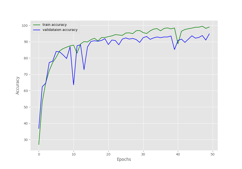
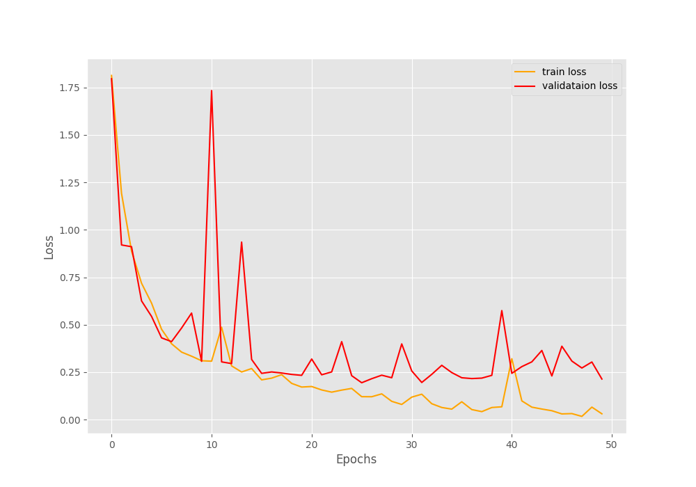
From the accuracy graph, it is pretty clear that both, the training and validation accuracy were increasing till the end of training. But we can see that the validation loss was starting to increase a bit after around 35 epochs. And most probably, this could be controlled by using a learning rate scheduler.

But all in all, it seems that the hyperparameter search actually worked. Instead of random experiments, we ran a Grid Search and the best hyperparameters seem to be working really well.

A Few Pros and Cons

Let’s take a look at the advantages we gained here over the last experiment when we did the manual hyperparameter search.

• We did not have to carry out any experiments manually. Everything was done by the hyperparameter search and it gave us the best ones for the 224×224 image dimensions.
• We got really good results by training with the best hyperparameters and on 224×224 images. Also, the training time for each epoch reduced.
• Combining that with proper regularization like, image augmentation, and learning rate scheduler will surely beat the manual method by a good margin.

Now, some of the disadvantages.

• The hypermeter search can take a lot of time. For only 2 batches of data, it took around 3 hours on an 10th Gen i7 CPU. More batches of data will give better search results, and can effectively take a up a day (or even more) for the search to complete if we condifer the entire dataset. Perhaps, this is one of the major disadvantages of hyperparameter search using PyTorch and Skorch where we are not able to use GPU for Grid Search.
• Everyone might not have the time or resources to carry out hyperparameter searches.
• Grid Search is not the best method for hyperparameter search as well. This we discussed in the last post and was discovered by James Bergstra and Yoshua Bengio and was published by them in the paper Random Search for Hyper-Parameter Optimization. Random Search performs better.

A Few Further Steps to Take

• Try out including different optimizer as well in the hyperparameter search.
• Maybe inlcuding more values for output channels and features for the neural network will also give better search results.
• And using learning rate scheduler is also a good next step.

If you try out any of the above be sure to let others know in the comment section about your results. Also, including more parameters in the hyperparameter search will surely increase the search time. So, you need to be a bit careful in that regard. Also, a hyperparameter search with PyTorch and Skorch may not be the best way. There are better libraries for this. And we will be taking a look at those in future posts.

Summary and Conclusion

In this post, you learned how to carry out hyperparameter search using PyTorch and Skorch. We used Grid Search to search for the best hyperparameters. We also trained our neural network with the best hyperparameters and noticed a few improvements over the manual search method. Finally, we ended the post with the advantages and disadvantages of the Grid Search method and hyperparameter search in general along with what we can do next. I hope that this tutorial was helpful to you.

If you have any doubts, thoughts, or suggestions, please leave them in the comment section. I will surely address them.

You can contact me using the Contact section. You can also find me on LinkedIn, and X.