Convolutional Neural Network in TensorFlow

In this tutorial, you will build your first convolutional neural network in TensorFlow.

This tutorial is the fifth in the series, Getting Started with TensorFlow.

• Introduction to Tensors in TensorFlow.
• Basics of TensorFlow GradientTape.
• Linear Regression using TensorFlow GradientTape.
• Training Your First Neural Network in TensorFlow.
• Convolutional Neural Network in TensorFlow.

In the last post, we learned how to build our first neural network in TensorFlow. We trained a Densely connected neural network on the MNIST Handwritten Digits and the Fashion MNIST dataset.

In this tutorial, we will take our learning one step further in deep learning with TensorFlow. Here, we will train a convolutional neural network on a standard image dataset.

We will cover the following topics in this tutorial.

• First, we will discuss how convolutional neural networks work.
• Then we will get to know a bit about the dataset that we will use, i.e., the CIFAR10 dataset.
• We will build our convolutional neural network in TensorFlow and train it on the CIFAR10 datasets.
• Finally, we will test it and check on which type of images it is making mistakes and which it is able to classify easily.

How Convolutional Neural Networks Work?

For any convolutional neural network, the convolutional layer is the most basic block. The main advantage they have over densely connected networks is that they preserve the spatial information of an image while extracting the features. There are mainly three things we need to know about when getting started with CNNs.

• Local Receptive Field.
• Feature Maps.
• Pooling Layer.

All other concepts will slowly build up when you explore computer vision and deep learning more.

Local Receptive Field in CNN

The local receptive field is a small area upon which the neurons of a CNN focus on. Different neurons focus on different areas of an image to extract the features and give us the feature map.

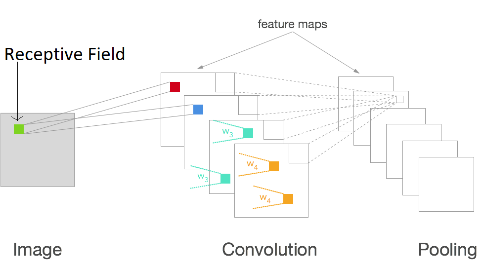
Feature Map

When all the neurons focus on their receptive fields, they extract the respective features out of the image pixels. Stacking these feature one after the other will give us a feature map as you see in figure 1.

And in terms of deep learning, we call each feature map a channel. So, after one convolution operation, if we have 10 feature maps, then we say that we have 10 channels.

Pooling Layer

The pooling layer helps in downsampling the obtained feature map. There a few types of pooling to get started with, namely:

• Max pooling.
• Average pooling.

In the case of max pooling, we take the maximum values out of a feature map over a specific pooling area.

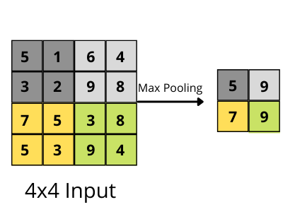
In figure 2, we have a max-pooling layer with kernel size 2×2 and stride 2. And you can see each 2×2 kernel extracts the maximum value out of the feature map area it is being applied on.

And in the case of average pooling, we average the values over the pooling area.

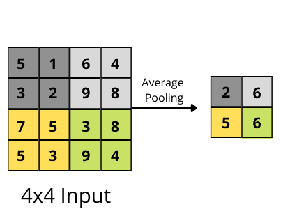
You can see that the final feature map after the average pooling operation contains the average values from the pooling area.

The above were some very basic explanations of the operations we need to consider when building a convolutional neural network. To get a much descriptive idea, please visit this link.

The CIFAR10 Dataset

As discussed earlier, we will use the CIFAR10 dataset in this tutorial to train a convolutional neural network. The CIFAR10 dataset is much more complex than what we used in the previous post.

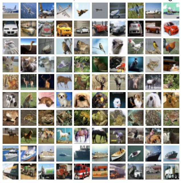
The images in CIFAR10 are RGB images having three color channels instead of 1. And all the images are resized to 32×32 dimensions. So, each image is 32x32x3 in dimension.

The images in the CIFAR10 dataset belong to 10 different classes. They are:

• Airplane => class 1.
• Automobile => class 2.
• Bird => class 3.
• Car => class 4.
• Deer => class 5.
• Dog => class 6.
• Frog => class 7.
• Horse => class 8.
• Ship => class 9.
• Truck => class 10.

There are 60000 images in total, so, 6000 per class. Out of these, 50000 are training examples and 10000 are test examples.

There is also a CIFAR100 dataset with 100 classes instead of 10. It contains 600 images for each class. But we will refrain from using this dataset for now as it is more difficult to tackle when compared with the CIFAR10 dataset. And in this Getting Started with TensorFlow series, we are learning new concepts. So, let’s keep things simple when starting out.

There is one more benefit of using the CIFAR10 dataset. It is also a part of

tf.keras.datasets module. So, we can download and use it with only one line of code.

Directory Strucutre

Let’s follow a simple directory structure for this project.

├── cifar10.ipynb

We have only a single Jupyter Notebook, that is,

cifar10.ipynb. We will write the code in this notebook and keep on visualizing the outputs as we execute each code cell. This is a great way of learning.

If you decide to code along while following the tutorial, I recommend using Jupyter Notebook as well. But if you are more comfortable with using Python scripts, then surely go ahead.

Apart from this notebook, a few other output images will be generated while executing the code. All of these will be saved in the same directory.

We have covered enough theory and preliminary stuff. Let’s jump into the coding part of the tutorial now.

Convolutional Neural Network in TensorFlow

While writing the code, we will divide each part into a sub-section to break it down into smaller chunks. And all the code will go into the

cifar10.ipynb file.

Let’s start with the import statements.

import tensorflow as tf
import numpy as np
import matplotlib.pyplot as plt
import matplotlib
import numpy as np

from sklearn.metrics import classification_report

matplotlib.style.use('ggplot')

We need

matplotlib for visualizing images and plotting graphs. And we will use classification_report from sklearn.metrics to check the precision, recall, and f1-score on the test set.

Import the CIFAR10 Dataset

Earlier we discussed that we can load the CIFAR10 dataset easily using the

tf.keras.datasets. Let’s do that and prepare the training and test set.

cifar10 = tf.keras.datasets.cifar10
(x_train, y_train), (x_test, y_test) = cifar10.load_data()
print(f"Number of training images: {len(x_train)}")
print(f"Number of test images: {len(x_test)}")
print(y_train)

If you have gone through the previous post, then you will find that the procedure is very similar to what we did in the case of the MNIST and Fashion MNIST dataset.

x_train and y_train hold the training images and corresponding labels, and x_test and y_test hold the test images and labels.

And printing

y_train gives the following output.

[[6]
 [9]
 [9]
 ...
 [9]
 [1]
 [1]]

The labels are numbered from 0 to 9 and we do not have any class name information. So, while visualizing the images, we will only be seeing the image and its corresponding label number, at least in the current state. Let’s create a list containing all the class names which we can map to the label numbers.

class_names = ['airplane', 'automobile', 'bird', 'cat', 'deer',
               'dog', 'frog', 'horse', 'ship', 'truck']

The

class_names list contains all the class names from the CIFAR10 dataset.

Visualize and Preprocess the Data

The following code block contains the code to visualize the first image from the training set.

plt.imshow(x_train[0])
plt.colorbar()
plt.savefig('cifar10-single-image.jpg')
plt.show()

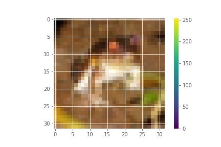
Most probably, the above image is of a frog. Note that we have not used the class names from the

class_names list and it is difficult for us to properly recognize the image. Let’s visualize a few more images, but this time with the proper class names.

Before that, let’s normalize the image pixels so that they would range between 0 and 1.

x_train = x_train / 255.0
x_test = x_test / 255.0

And now, visualizing a few images in subplot format.

plt.figure(figsize=(12, 9))
for i in range(9):
    plt.subplot(3, 3, i+1)
    plt.axis('off')
    plt.imshow(x_train[i])
    plt.colorbar()
    plt.title(class_names[int(y_train[i])])
plt.savefig('cifar10-images-with-labels.jpg')
plt.show()

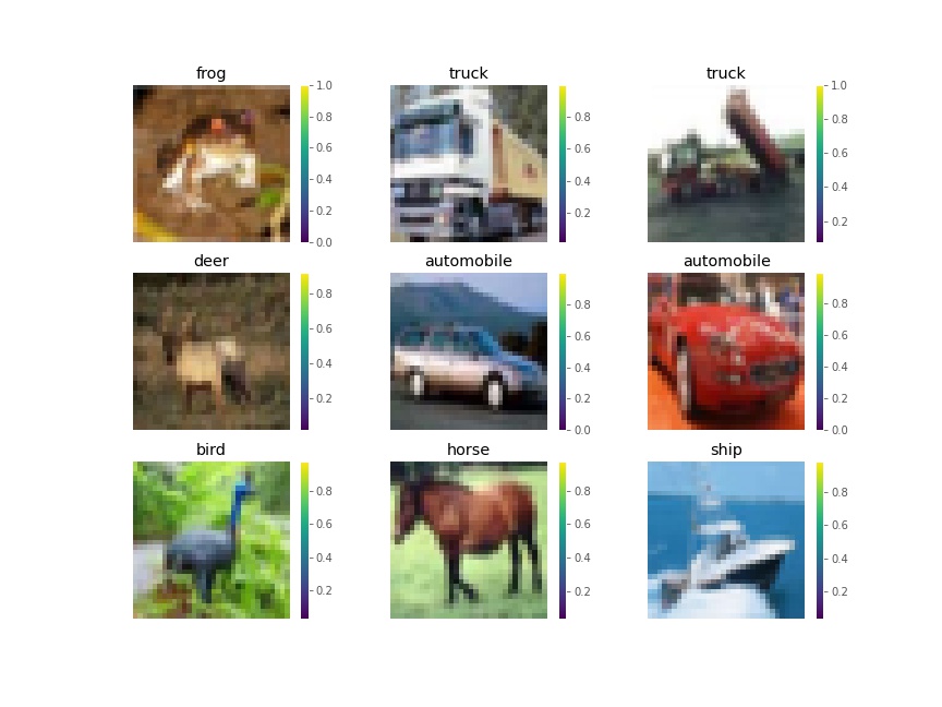
Much better! This time, we can clearly tell which image belongs to which class. And indeed, the previous image was that of a frog. Also, notice how all the image pixel values are between 0 and 1 now.

Build and Train the Neural Network Model

In this section, we will:

• Build the convolutional neural network model in TensorFlow.
• Compile it while providing the appropriate optimizer, loss function, and evaluation metric.
• And train the model as well.

Stack the Neural Network Layers

To tackle the problem, we will build a convolutional neural network. Our neural network model will mostly consist of 2D convolutional layers, 2D max-pooling layers, and Dense (linearly connected) layers.

It is going to be a simple network. As we are just starting to learn and build convolutional neural networks, we need not dive into complex models. A simple model with easy to understand architecture will speed up our learning and understanding of the whole process as well.

We will use

tf.keras.Sequential to build our model.

model = tf.keras.Sequential([
    tf.keras.layers.Conv2D(filters=32, kernel_size=(3, 3), activation='relu', 
                           input_shape=(32, 32, 3)),
    tf.keras.layers.MaxPooling2D(pool_size=(2, 2), strides=2),
    tf.keras.layers.Conv2D(filters=64, kernel_size=(3, 3), activation='relu'),
    tf.keras.layers.MaxPooling2D(pool_size=(2, 2), strides=2),
    tf.keras.layers.Conv2D(filters=128, kernel_size=(3, 3), activation='relu'),
    tf.keras.layers.Flatten(),
    tf.keras.layers.Dense(128, activation='relu'),
    tf.keras.layers.Dense(10)
])

print(model.summary())

• The first layer is a
  Conv2D
  Conv2D layer. It accepsts a few arguments. The
  filters
  filters argument is the number of neurons that we want in the layer, which is 32 in our case. Then we have the
  kernel_size
  kernel_size which corresponds to the filter’s width and height. It is 3×3 in this case. The activation function is
  relu
  relu. Finally, the
  input_shape
  input_shape is
  (32, 32, 3)
  (32, 32, 3) as we know that each image in the dataset is 32×32 in size with 3 color channels.
• Then we have a
  MaxPooling2D
  MaxPooling2D layer. The
  pool_size
  pool_size is the window size over which to take the maximum value from. And the
  stride
  stride represents how far to the left and bottom will the window move for each pooling step.
• After that, we have one more
  Conv2D
  Conv2D, one
  MaxPooling2D
  MaxPooling2D, and another
  Conv2D
  Conv2D with increasing number of filters for the convolutional layers each time.
• Then we flatten the features before feeding them to a
  Dense
  Dense layer with 128 units.
• The final Dense layer contains 10 units as we have 10 classes in total.

The following is the network summary.

Model: "sequential"
_________________________________________________________________
Layer (type)                 Output Shape              Param #   
=================================================================
conv2d (Conv2D)              (None, 30, 30, 32)        896       
_________________________________________________________________
max_pooling2d (MaxPooling2D) (None, 15, 15, 32)        0         
_________________________________________________________________
conv2d_1 (Conv2D)            (None, 13, 13, 64)        18496     
_________________________________________________________________
max_pooling2d_1 (MaxPooling2 (None, 6, 6, 64)          0         
_________________________________________________________________
conv2d_2 (Conv2D)            (None, 4, 4, 128)         73856     
_________________________________________________________________
flatten (Flatten)            (None, 2048)              0         
_________________________________________________________________
dense (Dense)                (None, 128)               262272    
_________________________________________________________________
dense_1 (Dense)              (None, 10)                1290      
=================================================================
Total params: 356,810
Trainable params: 356,810
Non-trainable params: 0
_________________________________________________________________
None

As you can see, the model has a total of 356,810 trainable parameters.

Compile the Model

To compile the model we will use the Adam optimizer, Sparse Categorical Cross-Entropy loss function, and accuracy as the evaluation metric. Let’s write the code for that.

model.compile(
    optimizer='adam',
    loss=tf.keras.losses.SparseCategoricalCrossentropy(from_logits=True),
    metrics=['accuracy']
)

Train the Model

Finally, we are all set to train the model. We will train the model for 10 epochs and save the accuracy and loss results in the

history variable.

history = model.fit(x_train, y_train, epochs=10)

Epoch 1/10
1563/1563 [==============================] - 19s 10ms/step - loss: 1.4646 - accuracy: 0.4673
Epoch 2/10
1563/1563 [==============================] - 16s 10ms/step - loss: 1.0923 - accuracy: 0.6137
Epoch 3/10
1563/1563 [==============================] - 16s 10ms/step - loss: 0.9183 - accuracy: 0.6781
Epoch 4/10
1563/1563 [==============================] - 16s 10ms/step - loss: 0.8191 - accuracy: 0.7126
Epoch 5/10
1563/1563 [==============================] - 16s 10ms/step - loss: 0.7352 - accuracy: 0.7418
Epoch 6/10
1563/1563 [==============================] - 16s 10ms/step - loss: 0.6654 - accuracy: 0.7669
Epoch 7/10
1563/1563 [==============================] - 17s 11ms/step - loss: 0.5935 - accuracy: 0.7909
Epoch 8/10
1563/1563 [==============================] - 16s 10ms/step - loss: 0.5319 - accuracy: 0.8145
Epoch 9/10
1563/1563 [==============================] - 16s 10ms/step - loss: 0.4737 - accuracy: 0.8318
Epoch 10/10
1563/1563 [==============================] - 16s 10ms/step - loss: 0.4129 - accuracy: 0.8529

After training for 10 epochs, the training accuracy is 85.29% and training loss is 0.4129. This seems just ok for starting out. We will get more insights when we evaluate the model on the test set and check the classification report for the same.

Plot the Accuracy and Loss Line Graphs

For now, we will plot the accuracy and loss line graphs. We can access the accuracy and loss values for all 10 epochs from the

history variable’s history dictionary which holds loss and accuracy as two keys.

train_loss = history.history['loss']
train_acc = history.history['accuracy']

# accuracy plot
plt.figure(figsize=(10, 7))
plt.plot(
    train_acc, color='green', linestyle='-', 
    label='train accuracy'
)
plt.xlabel('Epochs')
plt.ylabel('Accuracy')
plt.legend()
plt.savefig('cifar10-accuracy.jpg')
plt.show()
# loss plot
plt.figure(figsize=(10, 7))
plt.plot(
    train_loss, color='orange', linestyle='-', 
    label='train loss'
)
plt.xlabel('Epochs')
plt.ylabel('Loss')
plt.legend()
plt.savefig('cifar10-loss.jpg')
plt.show()

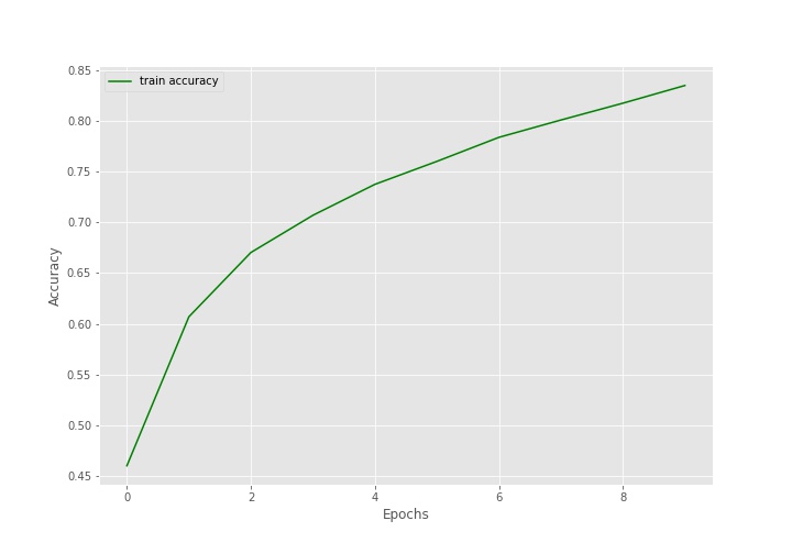
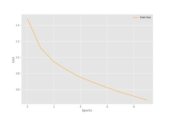
The above loss and accuracy plots also correspond to what we saw above while training. But it seems that training for more epochs is surely going to improve the model as the accuracy curve is still going higher up. So, the accuracy is not plateaued yet.

Evaluation Accuracy and Loss on the Test Set

We still have our test set that we have not used yet. Let’s evaluate our model on the test set and generate the classification report for the results.

test_loss, test_acc = model.evaluate(x_test, y_test, verbose=1)
print(f"Test accuracy: {test_acc*100:.3f}")
print(f"Test loss: {test_loss:.3f}")

Test accuracy: 72.420
Test loss: 0.982

The test accuracy is 72.42% and the test loss is 0.982. Clearly, the model is not that well trained by now. Training for more epochs will surely help and that was also what we inferred from looking at the graphs above.

The following code block generates the classification report.

y_pred = model.predict_classes(x_test)
cls_report = classification_report(y_test, y_pred)

for i in range(len(class_names)):
    print(f"Class {i}: {class_names[i]}")
print(cls_report)

Class 0: airplane
Class 1: automobile
Class 2: bird
Class 3: cat
Class 4: deer
Class 5: dog
Class 6: frog
Class 7: horse
Class 8: ship
Class 9: truck
              precision    recall  f1-score   support

           0       0.81      0.70      0.75      1000
           1       0.82      0.86      0.84      1000
           2       0.70      0.57      0.63      1000
           3       0.61      0.44      0.51      1000
           4       0.68      0.68      0.68      1000
           5       0.58      0.70      0.64      1000
           6       0.67      0.89      0.77      1000
           7       0.80      0.73      0.77      1000
           8       0.82      0.83      0.82      1000
           9       0.76      0.84      0.80      1000

    accuracy                           0.72     10000
   macro avg       0.73      0.72      0.72     10000
weighted avg       0.73      0.72      0.72     10000

It seems that the model is performing worst for the

dog class, followed by frog and deer.

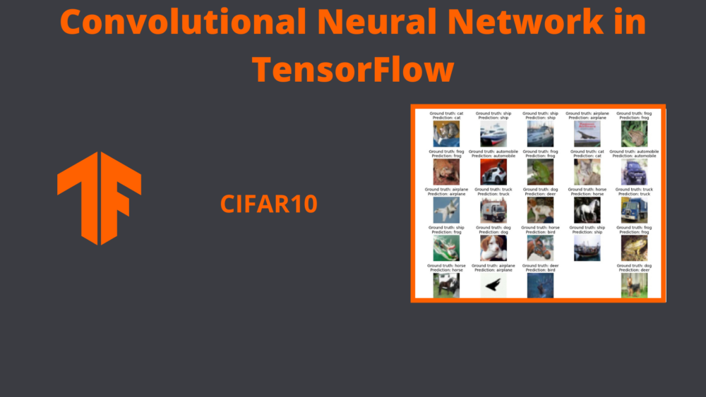
Visualize the Ground Truth and Prediction Labels for the Test Set

We can know which classes the model is predicting wrongly and what it is predicting for those classes by checking out a few ground truth and prediction labels for the test set.

Let’s write a simple code snippet to check those out.

plt.figure(figsize=(13, 10))
for i in range(25):
    plt.subplot(5, 5, i+1)
    plt.axis('off')
    plt.imshow(x_test[i])
    gt_string = f"Ground truth: {class_names[int(y_test[i])]}"
    pred_string = f"Prediction: {class_names[int(y_pred[i])]}" 
    plt.title(f"{gt_string}\n{pred_string}")
    plt.tight_layout()
plt.savefig('cifar10-test-gt-vs-pred-labels.jpg')
plt.show()

The above code will plot the first 25 images in the test. Along with that it will show the ground truth labels and the corresponding model predictions for those images. We can get some insights into what the model is predicting wrongly.

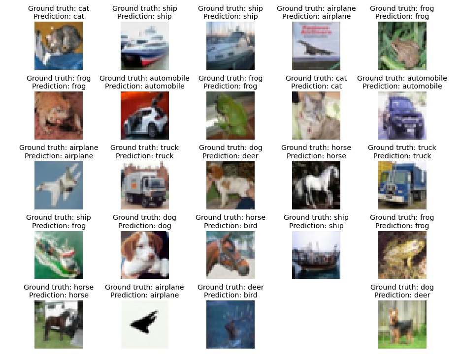
We can clearly see the model predicting wrongly for the

dog class. For the dog, it is mostly predicting as deer. And there are few wrong predictions for the horse and ship class as well.

Note: There is a chance that you might get different results for predictions as the learning might vary across different runs.

Clearly, we should train for more epochs and check whether the performance of the model improves or not.

A Few Takwaways

• We saw that to tackle complex images we need a more sophisiticated model as well. And for images, convolutional neural networks are a great solution.
• From the above experiment, we came to know that we may not always get the desired results in the first pass. We need to change our strategy a bit after looking at the initial results.
• Maybe training for more epochs is one of those things. You should surely try training the model for more epochs and tell about your findings in the comment section.
• Try building a more complex and larger model with more convolutional layers as well and see how it affects the accuracy. Beaware though, a larger model will also take longer to train.

Summary and Conclusion

In this tutorial, you learned how to build and train a convolutional neural network in TensorFlow. You trained a convolutional neural network on the CIFAR10 dataset and checked the performance on the test set. You also saw how we may not get very good results and need to experiment with the training and the model. I hope that you learned something new from this tutorial.

If you have any doubts, thoughts, or suggestions, then please leave them in the comment section. I will surely address them.

You can contact me using the Contact section. You can also find me on LinkedIn, and Twitter.