Fine Tuning Phi 1.5 using QLoRA

Quantized LoRA, more commonly known as QLoRA is a combination of quantization and Low Rank Adaptation for fine-tuning LLMs. Simply put, LoRa is a technique to adapt Large Language Models to specific tasks without making them forget their pretraining knowledge. In QLoRa, we load the pretrained model weights in quantized format, say 4-bit (INT4). However, the adapter (LoRA) layers are loaded in full precision, FP16 or FP32. This reduces the memory (GPU) consumption by a great extent making fine tuning possible on low resource hardware. To this end, in this article, we will be fine tuning the Phi 1.5 model using QLoRA.

We will use a combination of several libraries such as bitsandbytes, transformers, trl, and the PyTorch framework. For the QLoRA fine tuning task, we will use the Microsoft Phi 1.5 model which is a 1.3 billion parameter model. Best of all, we can do this on a 10 GB RTX 3080 GPU.

We will cover the following topics in this article

• We will start with a short discussion of the Stanford Alpaca Instruction Tuning dataset.
• Then we will move to the coding part:
  • First, we will cover the dataset and training configuration.
  • Second, we will load and prepare the model along with LoRA.
  • Third, we will fine tuning the Phi 1.5 model using QLoRA.
  • Finally, we will carry out inference using the trained model.

Note: We will not go into the theoretical details of LoRA and QLoRA in this article. However, we will do that in a future article.

What is The Stanford Alpaca Dataset?

The Stanford Alpaca dataset was primarily built to train the Llama model for instruction following. However, it has become one of the major datasets for prototyping and also fine-tuning various LLMs for instruction tuning. Check out the Instruction Tuning GPT2 on Alpaca Dataset to know how we can fine tune a GPT2 model on the same dataset.

The Stanford Alpaca dataset is available on GitHub as we all on Hugging Face datasets. Here, we will use the Hugging Face datasets for easier download and processing.

The dataset contains 52000 samples of instruction and response pairs. Observing the Hugging Face datasets uncovers two things:

• There are four columns in the dataset
• The final text column is a modified combination of the first three

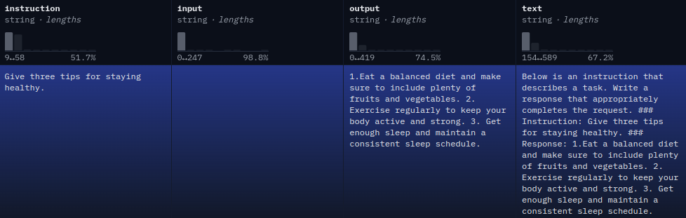
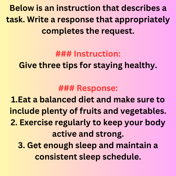
There are two possibilities for the text column instruction-input-output combination. The instruction may follow an empty input text.

Below is an instruction that describes a task. Write a response that appropriately completes the request. ### Instruction: Give three tips for staying healthy. ### Response: 1.Eat a balanced diet and make sure to include plenty of fruits and vegetables. 2. Exercise regularly to keep your body active and strong. 3. Get enough sleep and maintain a consistent sleep schedule.

Or there may be an input text after the instruction.

Below is an instruction that describes a task, paired with an input that provides further context. Write a response that appropriately completes the request. ### Instruction: Classify the following into animals, plants, and minerals ### Input: Oak tree, copper ore, elephant ### Response: Oak tree: Plant Copper ore: Mineral Elephant: Animal

If there is no input, then the input column remains empty. Later in the coding part, we will structure the input to the model in a particular manner depending on whether there is an input.

Project Directory Structure

Following is the directory structure of the project.

├── outputs
│   └── phi_1_5_alpaca_qlora
│       ├── best_model
│       │   ├── adapter_config.json
│       │   ├── adapter_model.safetensors
│       │   ├── added_tokens.json
│       │   ├── merges.txt
│       │   ├── README.md
│       │   ├── special_tokens_map.json
│       │   ├── tokenizer_config.json
│       │   └── vocab.json
│       └── logs
│           ├── checkpoint-274
│           └── runs
├── inference.ipynb
├── phi_1_5_alpaca_qlora.ipynb
└── requirements.txt

• We have two Jupyter Notebooks. The phi_1_5_alpaca_qlora.ipynb is for training and inference.ipynb contains the inference code.
• The outputs directory contains the best model, the final checkpoint, and the training logs.
• Also, we have a requirements file for installing all the necessary libraries.

The best-trained checkpoints and the training, and inference notebooks are downloadable via the download section. You can directly run inference if you wish to.

Dependencies

There are a few major libraries that we need to install before moving forward. The base framework is PyTorch.

• accelerate
• transformers
• trl
• datasets
• bitsandbytes
• peft

We can install all of these via the requirements.txt file.

pip install -r requirements.txt

That’s all we need for the setup. Now, let’s move to the coding part.

Download Code

Fine Tuning Phi 1.5 using QLoRA

The Phi 1.5 model by Microsoft is a 1.3 billion parameter model. Although far smaller than what we consider LLMs today, it is still difficult to do a full fine-tuning of the model on a single GPU. However, as we will see here, with QLoRA, we can do so with a 10 GB RTX 3080 GPU.

All the training code shown here is in the phi_1_5_alpaca_qlora.ipynb notebook.

The Import Statements

As always, first, we need to import all the necessary libraries and modules.

import os
import torch

from datasets import load_dataset
from transformers import (
    AutoModelForCausalLM,
    AutoTokenizer,
    TrainingArguments,
    pipeline,
    logging,
    BitsAndBytesConfig
)
from trl import SFTTrainer
from peft import LoraConfig

There are a few very important imports in the above code block:

• BitsAndBytesConfig from transformers: We need this for loading the model in 4-bit quantized format.
• SFTTrainer from trl: The Supervised Fine-Tuning Trainer pipeline helps us easily train LLMs for instruction following and chat.
• LoraConfig from peft: We need this for initializing the LoRA configuration.

Dataset and Training Configuration

Let’s define some of the training and dataset configurations that we will use throughout the training process.

batch_size = 1
num_workers = os.cpu_count()
epochs = 1
bf16 = True
fp16 = False
gradient_accumulation_steps = 16
context_length = 1024
learning_rate = 0.0002
model_name = 'microsoft/phi-1_5'
out_dir = 'outputs/phi_1_5_alpaca_qlora'

• Some of the generic ones are the batch size, the number of parallel workers for data loaders, and the training epochs. Notice that we are using a batch size of 1 as we have a limited GPU memory of just 10 GB. Also training for 1 epoch should be more than enough for initial experiments.
• bf16 and fp16: We can either carry out the training process in BFloat16 or Float16 mixed precision format. bf16 is slightly more stable, and faster, and is supported by the newer NVIDIA RTX GPUs. If you are training on older hardware like GTX GPUs, or P100, consider using fp16.
• gradient_accumulation_steps: LLM training generally benefits from larger batch sizes. However, it is difficult to use large batch sizes on a 10 GB GPU. This is where the Gradient Accumulation Step comes in. Basically, it tells the training pipeline to do backpropagation after batch_size * gradient_accumulation_steps instead of every batch. That means, for us, the backpropagation will happen every 16 batches.
• context_length: This is another important consideration that needs to be weighed in carefully. The larger the sequence length, the more context the model sees at a time. Although it is now a norm to use a sequence or context length of 4096, we are using 1024 due to memory constraints.
• learning_rate: The learning rate is 0.0002 which is quite high for fine-tuning, however, works well for LoRA training.
• model_name and out_dir: The former is the Hugging Face repo name from where to download the model. The latter is the directory where all the model weights and logs will be saved.

Loading and Preparing the Stanford Alpaca Dataset

The next step is to load the Stanford Alpaca dataset.

dataset = load_dataset('tatsu-lab/alpaca')

print(dataset['train']['text'][0])

Following is a sample from the text column of the dataset.

We will divide the dataset into a training and evaluation set.

full_dataset = dataset['train'].train_test_split(test_size=0.05, shuffle=True)
dataset_train = full_dataset['train']
dataset_valid = full_dataset['test']
 
print(dataset_train)
print(dataset_valid)

After splitting, there are 49400 samples for training and 2600 samples for evaluation.

We will not directly use the dataset from the text column for training. Rather we will define a preprocessing function to bring the dataset to a specific format.

def preprocess_function(example):
    text = f"### Instruction:\n{example['instruction']}\n\n### Input:\n{example['input']}\n\n### Response:\n{example['output']}"
    return text

After going through this preprocessing step, every sample will look like the following (if the input is empty):

### Instruction:
Generate a new design for a product packaging.

### Input:


### Response:
The product packaging should be bright and vibrant to catch the eye of customers. It should be designed to be eye-catching yet simple. The font should be clear, easy to read, and stylish. It should have a modern, sleek look and be made from durable and environmentally friendly materials. The packaging should also have clear labeling of product information, such as ingredients, directions for use, and any warnings or other important information.

If the input is not empty:

### Instruction:
Determine if the statement is always true, sometimes true, or never true based on your knowledge and common sense.

### Input:
An elephant has more than two legs.

### Response:
Always true.

We will use the above preprocess_function in the SFT Trainer pipeline.

Loading the Phi 1.5 Model for Stanford Alpaca Fine Tuning

Before loading the model, we need to define the quantization configuration.

# Quantization configuration.
if bf16:
    compute_dtype = getattr(torch, 'bfloat16')
else: # FP16
    compute_dtype = getattr(torch, 'float16')

quant_config = BitsAndBytesConfig(
    load_in_4bit=True,
    bnb_4bit_quant_type='nf4',
    bnb_4bit_compute_dtype=compute_dtype,
    bnb_4bit_use_double_quant=True
)

First, we define the compute data type depending on whether we chose FP16 or BF16 earlier.

Second, we define the quantization configuration for which we use BitsAndBytesConfig.

We load the model in 4-bit quantized format. However, it is not exactly INT4, rather, it is NF4, which 4-bit NormatFloat which gives better performance for normally distributed weights. The bnb_4bit_use_double_quant uses a second quantization step for additional memory saving. You can find more details here.

Third, loading the model with the quantization configuration.

model = AutoModelForCausalLM.from_pretrained(
    model_name,
    quantization_config=quant_config
)

Printing the model and its parameters gives us the following results.

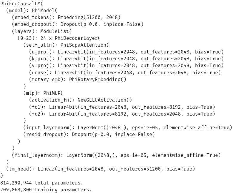
We can see right now that the total number of parameters and the trainable parameters have reduced. There is a very interesting reason for this, the details of which are out of the scope of this article. Please refer to this discussion thread to know more.

Loading the Tokenizer

Next, we will load the tokenizer.

tokenizer = AutoTokenizer.from_pretrained(
    model_name, 
    trust_remote_code=True,
    use_fast=False
)
tokenizer.pad_token = tokenizer.eos_token

The Phi 1.5 tokenizer does not contain a padding token by default. So, we set it to the EOS (End of Sequence) token.

Defining the Training Parameters and SFT Trainer

Before defining the training parameters, we also need to set the LoRA config.

peft_params = LoraConfig(
    lora_alpha=16,
    lora_dropout=0.1,
    r=16,
    bias='none',
    task_type='CAUSAL_LM',
) 

There are two major arguments in the above configuration, the LoRA rank r and lora_alhpa. The LoRA rank defines how large are the additional layers going to be. The larger the number, the more the training parameters. The LoRA Alpha determines how much the LoRA weights affect the model’s outputs. Most of the time, we can set both of them to the same value.

The next step is defining the training arguments.

training_args = TrainingArguments(
    output_dir=f"{out_dir}/logs",
    evaluation_strategy='epoch',
    weight_decay=0.01,
    load_best_model_at_end=True,
    per_device_train_batch_size=batch_size,
    per_device_eval_batch_size=batch_size,
    logging_strategy='epoch',
    save_strategy='epoch',
    num_train_epochs=epochs,
    save_total_limit=2,
    bf16=bf16,
    fp16=fp16,
    report_to='tensorboard',
    dataloader_num_workers=num_workers,
    gradient_accumulation_steps=gradient_accumulation_steps,
    learning_rate=learning_rate,
    lr_scheduler_type='constant',
)

I highly recommend going through the Instruction Tuning OPT-125M article, to get a detailed overview of the arguments used above.

Then, we need to define the SFT Trainer pipeline.

trainer = SFTTrainer(
    model=model,
    train_dataset=dataset_train,
    eval_dataset=dataset_valid,
    max_seq_length=context_length,
    tokenizer=tokenizer,
    args=training_args,
    packing=True,
    peft_config=peft_params,
    formatting_func=preprocess_function
)

We pass the peft_params and the preprocess_function while initializing SFTTrainer. There is one interesting observation though. Remember, how there were around 200 million trainable parameters earlier. However, we know that using LoRA training, only the adapter layers are trained. We get this if we print the parameters of the models now.

# Total parameters and trainable parameters.
total_params = sum(p.numel() for p in model.parameters())
print(f"{total_params:,} total parameters.")
total_trainable_params = sum(
    p.numel() for p in model.parameters() if p.requires_grad)
print(f"{total_trainable_params:,} training parameters.")

825,300,992 total parameters.
11,010,048 training parameters.

Now, there are just 11 million training parameters and all other weights are frozen in NF4 format.

Further, we can also check how the data loader has prepared the dataset.

dataloader = trainer.get_train_dataloader()
for i, sample in enumerate(dataloader):
    print(tokenizer.decode(sample['input_ids'][0]))
    print('#'*50)
    if i == 5:
        break

### Input:


### Response:
Climate change is causing extreme weather, sea level rise, drought, and deforestation, with damaging impact on humans and habitats.<|endoftext|>### Instruction:
Determine the next number in the following sequence: 10, 8, 6, 4...

### Input:


### Response:
2<|endoftext|>### Instruction:
Generate a new design for a product packaging.

### Input:


### Response:
The product packaging should be bright and vibrant to catch the eye of customers. It should be designed to be eye-catching yet simple. The font should be clear, easy to read, and stylish. It should have a modern, sleek look and be made from durable and environmentally friendly materials. The packaging should also have clear labeling of product information, such as ingredients, directions for use, and any warnings or other important information.<|endoftext|>### Instruction:
Create a research question related to the topic, "The Effects of Social Media on Mental Health".

### Input:

It just concatenates one sample after the other with an <|endoftext|> token after each sample.

Starting the Training Process

We can call the train method to start the training.

history = trainer.train()

trainer.model.save_pretrained(f"{out_dir}/best_model")
trainer.tokenizer.save_pretrained(f"{out_dir}/best_model")

Note that while saving a LoRA training best weights, we need to use trainer.model.save_pretrained instead of model.save_pretrained. This is quite important to save the weights correctly.

Analyzing the Phi 1.5 QLoRA Standford Alpaca Training Results

Let’s take a look at the training log here.

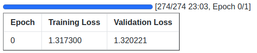
After the first epoch, the evaluation loss is 1.32.

Inference using the QLoRA Fine Tuned Phi 1.5 Model

Running inference, i.e., giving an instruction to the model and getting a response will reveal more about its capabilities.

The inference code is in the inference.ipynb notebook.

First, we need to import all the modules and load the model and the tokenizer.

from transformers import (
    AutoModelForCausalLM, 
    logging, 
    pipeline,
    AutoTokenizer
)

model = AutoModelForCausalLM.from_pretrained('outputs/phi_1_5_alpaca_qlora/best_model/')
tokenizer = AutoTokenizer.from_pretrained('outputs/phi_1_5_alpaca_qlora/best_model/')

Second, we define the text generation pipeline.

pipe = pipeline(
    task='text-generation', 
    model=model, 
    tokenizer=tokenizer, 
    max_length=256,
    eos_token_id=tokenizer.eos_token_id,
    device='cuda'
)

Third, we need to define a prompt in the same format as the training dataset after we had done our preprocessing.

prompt = """### Instruction:
What are LLMs?

### Input:


### Response:
"""

Finally, pass the prompt through the model to get the output.

result = pipe(
    prompt
)
print(result[0]['generated_text'])

Following is the output.

LLMs are a type of artificial intelligence that can learn and adapt to new situations. 
They are designed to be able to understand and respond to natural language, and can 
be used for a variety of tasks, such as customer service, language translation, and 
even medical diagnosis.

The result is not bad at all, considering we trained the Phi 1.5 model for just 1 epoch.

Let’s try correcting the grammar and spelling in a sentence where an input is followed by the instruction.

prompt = """### Instruction:
Correct the grammar and spelling of the following sentence.

### Input:
I am learn to drive a care.

### Response:
"""

result = pipe(
    prompt
)
print(result[0]['generated_text'])

We get the following output.

I am learning to drive a car.

Well, for simple grammar correction, the model is able to do it correctly.

Summary and Conclusion

We covered the QLoRA fine tuning of Phi 1.5 model on the Stanford Alpaca dataset in this article. Although we did not cover the theoretical concepts in detail, we covered the coding part extensively, starting from data preparation to inference. I hope this article was worth your time.

If you have any doubts, thoughts, or suggestions, please leave them in the comment section. I will surely address them.

You can contact me using the Contact section. You can also find me on LinkedIn, and Twitter.