SRCNN Implementation in PyTorch for Image Super Resolution

This tutorial is going to be really interesting and perhaps a bit big as well. In this tutorial, we will carry out the famous SRCNN implementation in PyTorch for image super resolution.

There are quite a good number of implementations of the SRCNN model in PyTorch for Image Super Resolution. A lot of them are open-source GitHub repositories with very good and advanced code. But there are very few blog posts/tutorials for the implementation of the SRCNN model in PyTorch. I think the main reason is the lengthy code-base and details that one needs to keep in mind. Anyways, we will be venturing into the same in this tutorial. This may not be the best (as compared to other GitHub repositories) or even the most exact reproduction of the paper (because of training time). But we will do the best that we can.

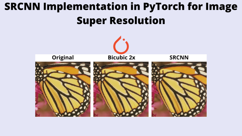
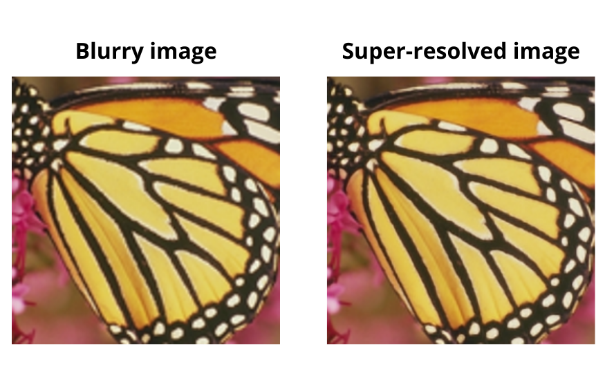
Just so that you may feel a bit motivated, the following is an example of the image super resolution as compared to the low resolution image.

What‘s special here? You may ask. Well, this is obtained using the exact code and trained model that we will cover in this tutorial. So, you can expect to achieve similar results when running inference using the same on your own low resolution images.

This is the second post in the SRCNN with PyTorch series.

• Image Super Resolution Using Deep Convolutional Networks: Paper Explanation
• SRCNN Implementation in PyTorch for Image Super Resolution

Points To Cover…

Let’s take a look at all the points that we will cover here:

• We will start with the preparation of the training dataset. We will use the same dataset as the paper, that is the T91 dataset.
• Next, we will prepare the validation datasets which are also the same as in the paper. These are the Set5 and Set14 datasets.
• Then, we will move on to the PyTorch dataset preparation code and training script. Here we will train our implementation of the SRCNN model in PyTorch with a few minor changes.
• After covering the training of the model, we will check out the super-resolved validation images that have been saved to the disk during the training. Comparing them to the low resolution images will give us a good idea of how well our model works.
• Finally, we will finish off with the takeaways from the project and further improvements.

Before we move further, there are a few points to keep in mind:

• If you want to know the details of the SRCNN paper, you may read the previous post. In that post, we discuss the Image Super-Resolution with Deep Convolutional Networks, the SRCNN architecture, and the experiment results in detail.
• As most of the theoretical aspects are already present in the previous post, in this tutorial, we will completely focus on the implementation and training of the SRCNN model in PyTorch.
• There are a few changes in the model and training pipeline as compared to the paper. We will discuss all of them in one of the further sections before jumping into the code.

SRCNN PyTorch Training Implementation Details

As discussed in one of the earlier points, our SRCNN model architecture implementation and the training pipeline will be slightly different. Let’s discuss them before moving any further into the coding section.

The SRCNN Model

In the paper, the original SRCNN model does not utilize padding. Therefore, the output is smaller compared to the input image. But in our implementation, we will use padding to ensure that the output image has the same shape as the input image. This is will make the implementation a bit simpler and also we can easily compare the input and output images. Also, the original model according to the paper (Caffe implementation) had 8,032 parameters. Although having the same architecture (except the padding), our PyTorch implementation of SRCNN will have a little over 20000 parameters.

The Learning Rate and Optimizer

The original implementation according to the paper uses the SGD optimizer with different learning rates for different layers. Here we use the Adam optimizer with the same learning rate for the entire model for easier implementation.

The Validation PSNR

We do not have a different PSNR calculation for the Set5 and Set14 datasets. Instead, we combine the Set5 and Set14 images into a single validation set and calculate the combined validation PSNR here. Although we will carry out final testing using both Set5 and Set14 datasets at the end to draw a comparison with the original results.

The Image Patches

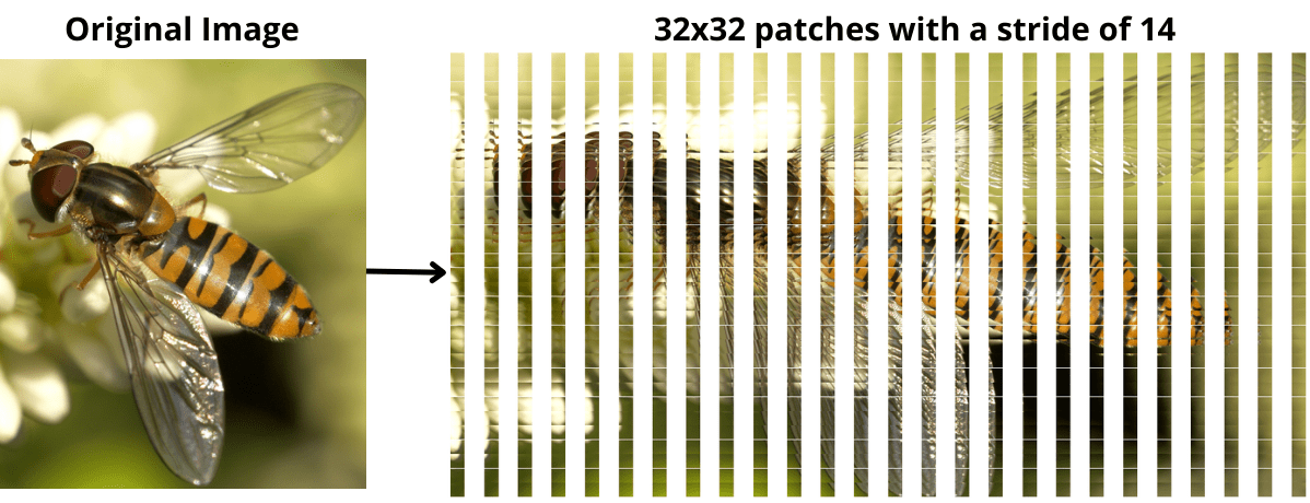
The authors extracted patches of size 32×32 from the T91 dataset with a stride of 14. This gave them 24,800 image patches. We will employ a similar strategy. But instead of writing manual code, we will use an open-source library. As we will see later on, we will end up with 22227 patches mostly because we do not finely control how the patches are being extracted. Still, this should not cause significant issues.

The Training Iterations

This is perhaps the most practical and compute-intensive part of this implementation.

The authors trained the SRCNN model for 8×10\(^8\) backpropagations. Now, that is quite a large number of iterations and it took them around three days on a GTX 770 GPU. It is impractical to do the same for a blog post. Still, we will train it for a large number of epochs, that is 2500 epochs with a batch size of 128. Now, that leaves us with around 432500 iterations in total. You need not worry about training it yourself as you can download the trained model with the zip file that is provided in this tutorial.

Download the Datasets

For this tutorial, we will need the T91, Set5, and Set14 datasets. These are very common image super resolution datasets. The paper used the above datasets and we will be doing the same.

You can find all the datasets among others in this Google Drive link.

You will also find a good amount of resources from the original author of the above datasets in the GitHub repository.

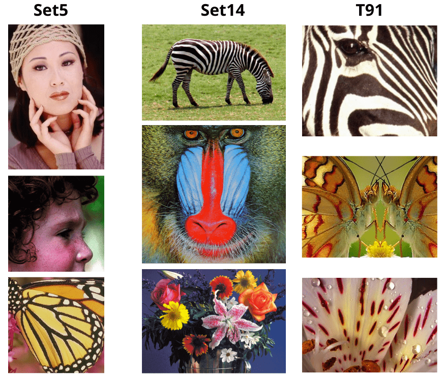
We will use the T91 dataset image patches for training which contains 91 images. The Set5 (containing 5 images) and Set14 (containing 14 images) datasets will be used for validation (during the training process) and later on for testing the trained model.

The following are a few images from each of the datasets.

You can download the three zip files from here and extract them yourself before executing any scripts. Or you may also use the ones that are provided with the downloadable file in this tutorial. In the later case, you need not extract anything as the datasets are already structured. The next section discusses the project directory structure.

Directory Structure

Let’s take a look at the directory structure of the project.

├── input
│   ├── Set14
│   ├── Set5
│   ├── T91
│   ├── t91_hr_patches
│   ├── t91_lr_patches
│   ├── test_bicubic_rgb_2x
│   ├── test_hr
│   ├── Set14.zip
│   ├── Set5.zip
│   └── T91.zip
├── outputs
│   ├── valid_results
│   ├── loss.png
│   ├── model_ckpt.pth
│   ├── model.pth
│   └── psnr.png
├── src
│   ├── bicubic.py
│   ├── datasets.py
│   ├── patchify_image.py
│   ├── srcnn.py
│   ├── test.py
│   ├── train.py
│   └── utils.py
└── NOTES.md

• The input directory: The input directory contains all the original training and validation datasets. This includes the zip files and the extracted data directories, which are T91, Set14, and Set5. Along with that, it also contains the training low resolution patches in t91_lr_patches, the training high resolution patches in t91_hr_patches, the low resolution validation images in test_bicubic_rgb_2x, and the high resolution validation images in test_hr. We will prepare all these image patches in the coding section of the tutorial.
• The outputs directory: This contains all the results from the training and validation loops. These include the loss and PSNR graphs, the model checkpoints and trained weights, and the output images from the validation loop (while training the model).
• The src directory: This directory contains all the Python source code files which we will discuss in the coding section.

Finally, the NOTES.md in the project root directory contains the steps to execute the required Python scripts to prepare the datasets and train the SRCNN model.

Library and Module Requirements

There are a few important libraries that you need to install before you can start the training locally.

• Here, we are using PyTorch as the deep learning framework. The code uses PyTorch 1.11.0. A slightly older version (>=1.9) should also work. You can install/upgrade your PyTorch version from here.
• We will use the patchify library to create the image patches. You can install it using the following command:

pip install patchify

• You will also need to install pillow library for resizing and applying bicubic interpolation to the images and image patches. Install it using the following command:

pip install Pillow

There are a few other common libraries that you can install as you move along with the code.

SRCNN Implementation in PyTorch for Image Super Resolution

We will start with the coding section of the tutorial from here onward.

Regarding the code explanation in the tutorial. We will try to go through as much explanation as possible. But as the implementation is pretty big and contains a lot of code, we will skip over a few general concepts.

We will cover all the Python code files in the following order:

• utils.py
• patchify_image.py
• bicubic.py
• datasets.py
• srcnn.py
• train.py

The above Python files contain all the code we need for training the SRCNN model. After training, we will test our trained model using the test.py script.

Also, please keep in mind that all the Python files will stay within the src directory.

Helper Functions and Utility Scripts

Let’s start with writing the helper functions that we will need along with the way. The code for helper functions and utilities will go inside the utils.py file.

The PSNR Metric Function

Starting with the import statements and the function to calculate PSNR (Peak Signal to Noise Ratio).

import math
import numpy as np
import matplotlib.pyplot as plt
import torch

from torchvision.utils import save_image

plt.style.use('ggplot')

def psnr(label, outputs, max_val=1.):
    """
    Compute Peak Signal to Noise Ratio (the higher the better).
    PSNR = 20 * log10(MAXp) - 10 * log10(MSE).
    https://en.wikipedia.org/wiki/Peak_signal-to-noise_ratio#Definition

    Note that the output and label pixels (when dealing with images) should
    be normalized as the `max_val` here is 1 and not 255.
    """
    label = label.cpu().detach().numpy()
    outputs = outputs.cpu().detach().numpy()
    diff = outputs - label
    rmse = math.sqrt(np.mean((diff) ** 2))
    if rmse == 0:
        return 100
    else:
        PSNR = 20 * math.log10(max_val / rmse)
        return PSNR

The psnr function defines the metric that we will use to monitor the SRCNN model while training. Basically, the PSNR value keeps on increasing as the difference between the output image from the network and the ground truth high resolution keeps on decreasing. It is a very common metric for estimating quality between image reconstructions. This can also be used in other practical problems like image deblurring and image restoration.

You can find more details about PSNR here.

Helper Function to Save Loss and PSNR Graphs

Next, we have the functions to save the loss and PSNR graphs for training and validation.

def save_plot(train_loss, val_loss, train_psnr, val_psnr):
    # Loss plots.
    plt.figure(figsize=(10, 7))
    plt.plot(train_loss, color='orange', label='train loss')
    plt.plot(val_loss, color='red', label='validataion loss')
    plt.xlabel('Epochs')
    plt.ylabel('Loss')
    plt.legend()
    plt.savefig('../outputs/loss.png')
    plt.close()

    # PSNR plots.
    plt.figure(figsize=(10, 7))
    plt.plot(train_psnr, color='green', label='train PSNR dB')
    plt.plot(val_psnr, color='blue', label='validataion PSNR dB')
    plt.xlabel('Epochs')
    plt.ylabel('PSNR (dB)')
    plt.legend()
    plt.savefig('../outputs/psnr.png')
    plt.close()

The save_plot function accepts the lists containing the loss and PSNR values for training & validation and saves the corresponding graphs to disk.

Helper Functions to Save Models

The next two helper functions are for saving the model state dictionary (weights only) and the model checkpoint.

def save_model_state(model):
    # save the model to disk
    print('Saving model...')
    torch.save(model.state_dict(), '../outputs/model.pth')

def save_model(epochs, model, optimizer, criterion):
    """
    Function to save the trained model to disk.
    """
    # Remove the last model checkpoint if present.
    torch.save({
                'epoch': epochs+1,
                'model_state_dict': model.state_dict(),
                'optimizer_state_dict': optimizer.state_dict(),
                'loss': criterion,
                }, f"../outputs/model_ckpt.pth")

In the above code block, the save_model_state function saves just the model state (trained weights) to the disk. We can use this for inference and share this as well because this will be smaller in size. On the other hand, save_model function, saves the entire model checkpoint to disk. This will save the state dictionary, the number of epochs trained for, the optimizer state dictionary, and the loss function as well. This will be a larger model because of the extra information but we can use this to resume training in the future if the case arises.

It is worthwhile to keep in mind that we will not save the model checkpoint after every epoch. In many cases, the checkpoints with all the extra information can be quite large and are therefore saved every few epochs. This is to ensure that even if we stop the training at some point we can resume it from a nearby checkpoint. Although our model is very small, still, we will employ the same strategy of saving it after a certain number of epochs instead of every epoch. We will see the details in the training script.

Helper Function to Save Validation Images to Disk

The final helper function saves the reconstructed images from the validation loop to the disk. This will give us a visual representation of how well our model is learning. Again, we will not be saving these reconstructed images after every epoch. We will save them every 500 epochs as per the training script.

def save_validation_results(outputs, epoch, batch_iter):
    """
    Function to save the validation reconstructed images.
    """
    save_image(
        outputs, 
        f"../outputs/valid_results/val_sr_{epoch}_{batch_iter}.png"
    )

That’s all the helper functions we need.

Preparing the T91 Training Dataset for SRCNN Implementation in PyTorch

In this section, we will create the low and high resolution image patches for the T91 training dataset.

We will use the patchify library for this which we discussed in one of the previous sections. The following are the details of creating the patches.

• We will take the original images from the T91 dataset.
• Then we will create 32×32 dimensional patches from them and save them to disk.
• We will also resize these patches to half their size and again upsample them to the original size. Both of them will use the bicubic interpolation which is in line with the original implementation. This will provide us the 2x upsampled bicubic blurry images for each of the original patches.
• Now, keep in mind that these blurry patches are the same resolution as the high resolution patches (32×32). We just call them low resolution for convenience.

Let’s take a look at the code for more understanding. The following code will go into the patchify_image.py file.

Imports and Constants

The first code block contains the import statements and a few constants.

from PIL import Image
from tqdm import tqdm

import matplotlib.pyplot as plt
import patchify
import numpy as np
import matplotlib.gridspec as gridspec
import glob as glob
import os
import cv2

SHOW_PATCHES = False
STRIDE = 14
SIZE = 32

We will use PIL for reading and resizing images. cv2 is for saving the patches to disk and matplotlib for visualizing the patches if needed. There are three constants as well. The SHOW_PATCHES stores a boolean value indicating whether we want to visualize the image patches while executing the code or not. It is better to keep it as False after visualizing a few patches as you will have to press a key on the keyboard every time an image pops up so that the code can move on to the next image. The other two constants define the patch size and stride.

The Required Functions

We have two important functions in this script. Let’s write them first, then we will go to the explanation part.

def show_patches(patches):
    plt.figure(figsize=(patches.shape[0], patches.shape[1]))
    gs = gridspec.GridSpec(patches.shape[0], patches.shape[1])
    gs.update(wspace=0.01, hspace=0.02)
    counter = 0
    for i in range(patches.shape[0]):
        for j in range(patches.shape[1]):
            ax = plt.subplot(gs[counter])
            plt.imshow(patches[i, j, 0, :, :, :])
            plt.axis('off')
            counter += 1
    plt.show()

def create_patches(
    input_paths, out_hr_path, out_lr_path,
):
    os.makedirs(out_hr_path, exist_ok=True)
    os.makedirs(out_lr_path, exist_ok=True)
    all_paths = []

    for input_path in input_paths:
        all_paths.extend(glob.glob(f"{input_path}/*"))
    print(f"Creating patches for {len(all_paths)} images")

    for image_path in tqdm(all_paths, total=len(all_paths)):
        image = Image.open(image_path)
        image_name = image_path.split(os.path.sep)[-1].split('.')[0]
        w, h = image.size
        # Create patches of size (32, 32, 3)
        patches = patchify.patchify(np.array(image), (32, 32, 3), STRIDE)
        if SHOW_PATCHES:
            show_patches(patches)

        counter = 0
        for i in range(patches.shape[0]):
            for j in range(patches.shape[1]):
                counter += 1
                patch = patches[i, j, 0, :, :, :]
                patch = cv2.cvtColor(patch, cv2.COLOR_RGB2BGR)
                cv2.imwrite(
                    f"{out_hr_path}/{image_name}_{counter}.png",
                    patch
                )

                # Convert to bicubic and save.
                h, w, _ = patch.shape
                low_res_img = cv2.resize(patch, (int(w*0.5), int(h*0.5)), 
                                        interpolation=cv2.INTER_CUBIC)

                # Now upscale using BICUBIC.
                high_res_upscale = cv2.resize(low_res_img, (w, h), 
                                            interpolation=cv2.INTER_CUBIC)
                cv2.imwrite(
                    f"{out_lr_path}/{image_name}_{counter}.png",
                    high_res_upscale
                )

The show_patches function accepts the image patches and displays them using Matplotlib if SHOW_PATCHES is True.

But all of the important operations happen in the create_patches function. On lines 31 and 32, we create the directories to save the low and high resolution image patches. Then we read and store all the original image patches using glob in the all_paths list.

While iterating over the image paths, first we read the images, extract the original height and width, and then create the patches using patchify on line 44. It takes the input image as an array, the patch size that we want along with the color channel, and the stride, which is 14 here as the arguments.

It will return a square matrix depending on the stride and patch size which will contain 32×32 dimensional images. We start iterating over the rows and columns of that matrix on lines 49 and 50. Then we extract each of the corresponding patches on line 52 and save it to disk using OpenCV after converting to BGR format.

We create the corresponding low resolution patch on line 61. Because we are using 2x bicubic upscaling (line 65) to again obtain the original size blurry path, so, we just multiply the width and height of the patch by 0.5 to downscale them. Finally, We save these low resolution (same 32×32 dimensional, but blurry) patches to disk as well.

The Main Code Block

And finally, the main code block while calling the create_patches function while passing the required paths as arguments.

if __name__ == '__main__':
    create_patches(
        ['../input/T91'],
        '../input/t91_hr_patches',
        '../input/t91_lr_patches'
    )

Execute the above script from the command line/terminal while being within the src directory.

python patchify_image.py

The output should be similar to the following.

Creating patches for 91 images
100%|████████████████████████████████████████████████████████████████████| 91/91 [00:06<00:00, 13.52it/s]

The following is an image along with its overlapping patches that are created by the above code.

Creating the Validation Images

For the validation loop, we will combine the images from the Set5 and Set14 datasets. We will not create any patches out of them. Instead, we will use the whole original images as the ground truth and the bicubic 2x upsampled low resolution images as the input.

The bicubic.py script prepares the validation dataset.

The following code block contains the import statements and the argument parsers.

from PIL import Image

import glob as glob
import os
import argparse

# Construct the argument parser and parse the command line arguments.
parser = argparse.ArgumentParser()
parser.add_argument('-p', '--path', default='../input/Set14/original', 
                    nargs='+',
                    help='path to the high-res images to convert to low-res')
parser.add_argument('-s', '--scale-factor', dest='scale_factor', default='2x', 
                    help='make low-res by how much factor', 
                    choices=['2x', '3x', '4x'])
args = vars(parser.parse_args())

The --path flag takes multiple paths as input and we will provide the paths to the Set5 and Set14 original images. And the --scale-factor flag defines the bicubic scale for downsampling and upscaling again. We will use the 2x scale factor.

The next block contains the rest of the code.

paths = args['path']
images = []
for path in paths:
    images.extend(glob.glob(f"{path}/*.png"))
print(len(images))

# Select scaling-factor and set up directories according to that.
if args['scale_factor'] == '2x':
    scale_factor = 0.5
    os.makedirs('../input/test_bicubic_rgb_2x', exist_ok=True)
    save_path_lr = '../input/test_bicubic_rgb_2x'
    os.makedirs('../input/test_hr', exist_ok=True)
    save_path_hr = '../input/test_hr'
if args['scale_factor'] == '3x':
    scale_factor = 0.333
    os.makedirs('../input/test_bicubic_rgb_3x', exist_ok=True)
    os.makedirs('../input/test_hr', exist_ok=True)
    save_path_lr = '../input/test_bicubic_rgb_3x'
    save_path_hr = '../input/test_hr'
if args['scale_factor'] == '4x':
    scale_factor = 0.25
    os.makedirs('../input/test_bicubic_rgb_4x', exist_ok=True)
    os.makedirs('../input/test_hr', exist_ok=True)
    save_path_lr = '../input/test_bicubic_rgb_4x'
    save_path_hr = '../input/test_hr'

print(f"Scaling factor: {args['scale_factor']}")
print(f"Low resolution images save path: {save_path_lr}")

for image in images:
    orig_img = Image.open(image)
    image_name = image.split(os.path.sep)[-1]
    w, h = orig_img.size[:]
    print(f"Original image dimensions: {w}, {h}")
    orig_img.save(f"{save_path_hr}/{image_name}")

    low_res_img = orig_img.resize((int(w*scale_factor), int(h*scale_factor)), Image.BICUBIC)
    # Upscale using BICUBIC.
    high_res_upscale = low_res_img.resize((w, h), Image.BICUBIC)
    high_res_upscale.save(f"{save_path_lr}/{image_name}")

From lines 23 to 40, we create the directories to save low and high resolution images as per the scale factor. The code contains the other options so that further experiments can be done easily.

Starting from lines 45 to 55, we read the image and save the original and bicubic interpolated images to the corresponding folders.

We need to execute the above script from the src directory using the following command.

python bicubic.py --path ../input/Set14/original ../input/Set5/original --scale-factor 2x

The following is the output.

Scaling factor: 2x
Low resolution images save path: ../input/test_bicubic_rgb_2x
Original image dimensions: 500, 480
...
Original image dimensions: 228, 344

This completes all the preprocessing needed for the datasets.

Creating the PyTorch Datasets and Data Loaders

Now, we will create the PyTorch datasets and data loaders. This part is going to be simple as we don’t need much pre-processing of the images.

This code will go into the datasets.py file.

First, we have the imports and the constants defining the training and test (validation batch size).

import torch
import numpy as np
import glob as glob

from torch.utils.data import DataLoader, Dataset
from PIL import Image

TRAIN_BATCH_SIZE = 128
TEST_BATCH_SIZE = 1

For training, we will use a batch size of 128. But the validation set contains only 19 images, so we use a batch size of 1. This will also make it easier for us to save the reconstructed validation images.

Next is the custom dataset class.

# The SRCNN dataset module.
class SRCNNDataset(Dataset):
    def __init__(self, image_paths, label_paths):
        self.all_image_paths = glob.glob(f"{image_paths}/*")
        self.all_label_paths = glob.glob(f"{label_paths}/*") 

    def __len__(self):
        return (len(self.all_image_paths))

    def __getitem__(self, index):
        image = Image.open(self.all_image_paths[index]).convert('RGB')
        label = Image.open(self.all_label_paths[index]).convert('RGB')

        image = np.array(image, dtype=np.float32)
        label = np.array(label, dtype=np.float32)

        image /= 255.
        label /= 255.

        image = image.transpose([2, 0, 1])
        label = label.transpose([2, 0, 1])

        return (
            torch.tensor(image, dtype=torch.float),
            torch.tensor(label, dtype=torch.float)
        )

The above is a very simple dataset class that reads the low resolution images (input) and the high resolution (ground truth labels) images. After reading the images in RGB format, we convert the images to NumPy array, scale them by dividing them by 255, transpose them to bring the channel dimension to the front, and return them as tensors.

The last two functions create the datasets and data loaders for training and validation.

# Prepare the datasets.
def get_datasets(
    train_image_paths, train_label_paths,
    valid_image_path, valid_label_paths
):
    dataset_train = SRCNNDataset(
        train_image_paths, train_label_paths
    )
    dataset_valid = SRCNNDataset(
        valid_image_path, valid_label_paths
    )
    return dataset_train, dataset_valid

# Prepare the data loaders
def get_dataloaders(dataset_train, dataset_valid):
    train_loader = DataLoader(
        dataset_train, 
        batch_size=TRAIN_BATCH_SIZE,
        shuffle=True
    )
    valid_loader = DataLoader(
        dataset_valid, 
        batch_size=TEST_BATCH_SIZE,
        shuffle=False
    )
    return train_loader, valid_loader

The get_datasets function accepts the training image paths, training ground truth label paths, validation image paths, and validation ground truth label paths. This returns the dataset_train and dataset_valid.

In the get_dataloaders function, we create the training and validation dataset loaders and return them.

The SRCNN Model Implementation in PyTorch

The SRCNN model is going to be really simple. The srcnn.py file will hold the code for that.

import torch.nn as nn
import torch.nn.functional as F

class SRCNN(nn.Module):
    def __init__(self):
        super(SRCNN, self).__init__()

        self.conv1 = nn.Conv2d(
            3, 64, kernel_size=9, stride=(1, 1), padding=(2, 2)
        )
        self.conv2 = nn.Conv2d(
            64, 32, kernel_size=1, stride=(1, 1), padding=(2, 2)
        )
        self.conv3 = nn.Conv2d(
            32, 3, kernel_size=5, stride=(1, 1), padding=(2, 2)
        )

    def forward(self, x):
        x = F.relu(self.conv1(x))
        x = F.relu(self.conv2(x))
        x = self.conv3(x)

        return x

As you can see, we are using the base architecture from the paper. And as discussed earlier, the only difference here is the extra padding to obtain the same size outputs as that of the input images.

The Training Script

We need to write the code for the training script before we can start the training. We will not need to go through much explanation here as most of the code has already been written and we just need to compile them together.

The training script code will go into the train.py file.

import torch
import time
import srcnn
import torch.optim as optim
import torch.nn as nn
import os
import argparse

from tqdm import tqdm
from datasets import get_datasets, get_dataloaders
from utils import (
    psnr, save_model, save_model_state, 
    save_plot, save_validation_results
)

We import all the required libraries along with the custom modules in the above code block.

The next code block contains the argument parsers, the learning parameters, and path constants.

parser = argparse.ArgumentParser()
parser.add_argument(
    '-e', '--epochs', default=100, type=int,
    help='number of epochs to train for'
)
parser.add_argument(
    '-w', '--weights', default=None,
    help='weights/checkpoint path to resume training'
)
args = vars(parser.parse_args())

# Learning parameters.
epochs = args['epochs'] # Number of epochs to train the SRCNN model for.
lr = 0.001 # Learning rate.
device = 'cuda' if torch.cuda.is_available() else 'cpu'

# Constants
TRAIN_LABEL_PATHS = '../input/t91_hr_patches'
TRAN_IMAGE_PATHS = '../input/t91_lr_patches'
VALID_LABEL_PATHS = '../input/test_hr'
VALID_IMAGE_PATHS = '../input/test_bicubic_rgb_2x'
SAVE_VALIDATION_RESULTS = True

os.makedirs('../outputs/valid_results', exist_ok=True)

The argument parser contains the following flags:

• --epochs: To specify the number of epochs to train for.
• --weights: Path to the previously trained weights if willing to resume training. But we will not use this flag in this tutorial.

We are using the learning rate of 0.001 and the computation device is cuda.

In the constants, we define the image paths and whether to save the validation reconstructed images or not using SAVE_VALIDATION_RESULTS. We will save these images in the outputs/valid_results directory.

Initialize the Model, Optimizer, Loss Function, and Define the Data Loaders

The next code block defines the model, the Adam Optimizer, and the MSE loss function.

# Initialize the model.
print('Computation device: ', device)
model = srcnn.SRCNN().to(device)
if args['weights'] is not None:
    print('Loading weights to resume training...')
    checkpoint = torch.load(args['weights'])
    model.load_state_dict(checkpoint['model_state_dict'])
print(model)

# Optimizer.
optimizer = optim.Adam(model.parameters(), lr=lr)
# Loss function. 
criterion = nn.MSELoss()

dataset_train, dataset_valid = get_datasets(
    TRAN_IMAGE_PATHS, TRAIN_LABEL_PATHS,
    VALID_IMAGE_PATHS, VALID_LABEL_PATHS
)
train_loader, valid_loader = get_dataloaders(dataset_train, dataset_valid)

print(f"Training samples: {len(dataset_train)}")
print(f"Validation samples: {len(dataset_valid)}")

As you may observe on line 42, if we provide a trained model path, then the weights are loaded after initializing the SRCNN model.

The Training and Validation Functions

Here, in the training and validation loops, we will calculate the PSNR metric and the MSE loss.

def train(model, dataloader):
    model.train()
    running_loss = 0.0
    running_psnr = 0.0
    for bi, data in tqdm(enumerate(dataloader), total=len(dataloader)):
        image_data = data[0].to(device)
        label = data[1].to(device)
        
        # Zero grad the optimizer.
        optimizer.zero_grad()
        outputs = model(image_data)
        loss = criterion(outputs, label)

        # Backpropagation.
        loss.backward()
        # Update the parameters.
        optimizer.step()

        # Add loss of each item (total items in a batch = batch size).
        running_loss += loss.item()
        # Calculate batch psnr (once every `batch_size` iterations).
        batch_psnr =  psnr(label, outputs)
        running_psnr += batch_psnr

    final_loss = running_loss/len(dataloader.dataset)
    final_psnr = running_psnr/len(dataloader)
    return final_loss, final_psnr


def validate(model, dataloader, epoch):
    model.eval()
    running_loss = 0.0
    running_psnr = 0.0
    with torch.no_grad():
        for bi, data in tqdm(enumerate(dataloader), total=len(dataloader)):
            image_data = data[0].to(device)
            label = data[1].to(device)
            
            outputs = model(image_data)
            loss = criterion(outputs, label)

            # Add loss of each item (total items in a batch = batch size) .
            running_loss += loss.item()
            # Calculate batch psnr (once every `batch_size` iterations).
            batch_psnr = psnr(label, outputs)
            running_psnr += batch_psnr

            # For saving the batch samples for the validation results
            # every 500 epochs.
            if SAVE_VALIDATION_RESULTS and (epoch % 500) == 0:
                save_validation_results(outputs, epoch, bi)

    final_loss = running_loss/len(dataloader.dataset)
    final_psnr = running_psnr/len(dataloader)
    return final_loss, final_psnr

Also, in the validation loop, we save all 19 reconstructed images every 500 epochs (line 110). We will be able to compare the results with the bicubic and original images after the training completes.

Finally, we need to train the model for the specified number of epochs.

train_loss, val_loss = [], []
train_psnr, val_psnr = [], []
start = time.time()
for epoch in range(epochs):
    print(f"Epoch {epoch + 1} of {epochs}")
    train_epoch_loss, train_epoch_psnr = train(model, train_loader)
    val_epoch_loss, val_epoch_psnr = validate(model, valid_loader, epoch+1)
    print(f"Train PSNR: {train_epoch_psnr:.3f}")
    print(f"Val PSNR: {val_epoch_psnr:.3f}")
    train_loss.append(train_epoch_loss)
    train_psnr.append(train_epoch_psnr)
    val_loss.append(val_epoch_loss)
    val_psnr.append(val_epoch_psnr)
    
    # Save model with all information every 100 epochs. Can be used 
    # resuming training.
    if (epoch+1) % 100 == 0:
        save_model(epoch, model, optimizer, criterion)
    # Save the model state dictionary only every epoch. Small size, 
    # can be used for inference.
    save_model_state(model)
    # Save the PSNR and loss plots every epoch.
    save_plot(train_loss, val_loss, train_psnr, val_psnr)

end = time.time()
print(f"Finished training in: {((end-start)/60):.3f} minutes") 

We print the training and validation PSNR after every epoch. Along with that, we also save the model checkpoint every 100 epochs and the model state dictionary after every epoch.

Execute the train.py Script

We are now all set to execute the train.py script from the src directory.

Note: The training was done using a P100 GPU with 16 GB of VRAM.

Execute the following command to start training.

python train.py --epochs 2500

The training on the P100 GPU took somewhere around 10 hours.

The following block shows the sample output.

Computation device:  cuda
SRCNN(
  (conv1): Conv2d(3, 64, kernel_size=(9, 9), stride=(1, 1), padding=(2, 2))
  (conv2): Conv2d(64, 32, kernel_size=(1, 1), stride=(1, 1), padding=(2, 2))
  (conv3): Conv2d(32, 3, kernel_size=(5, 5), stride=(1, 1), padding=(2, 2))
)
Training samples: 22227
Validation samples: 19
Epoch 1 of 2500
100%|█████████████████████████████████████████| 174/174 [00:17<00:00, 10.15it/s]
100%|███████████████████████████████████████████| 19/19 [00:00<00:00, 37.10it/s]
Train PSNR: 17.312
Val PSNR: 23.656
Saving model...
Epoch 2 of 2500
100%|█████████████████████████████████████████| 174/174 [00:10<00:00, 15.99it/s]
100%|███████████████████████████████████████████| 19/19 [00:00<00:00, 38.19it/s]
.
.
.
Epoch 2499 of 2500
100%|█████████████████████████████████████████| 174/174 [00:11<00:00, 14.54it/s]
100%|███████████████████████████████████████████| 19/19 [00:00<00:00, 35.62it/s]
Train PSNR: 29.856
Val PSNR: 29.651
Saving model...
Epoch 2500 of 2500
100%|█████████████████████████████████████████| 174/174 [00:12<00:00, 14.47it/s]
100%|███████████████████████████████████████████| 19/19 [00:02<00:00,  7.43it/s]
Train PSNR: 29.850
Val PSNR: 29.613
Saving model...
Finished training in: 551.823 minutes

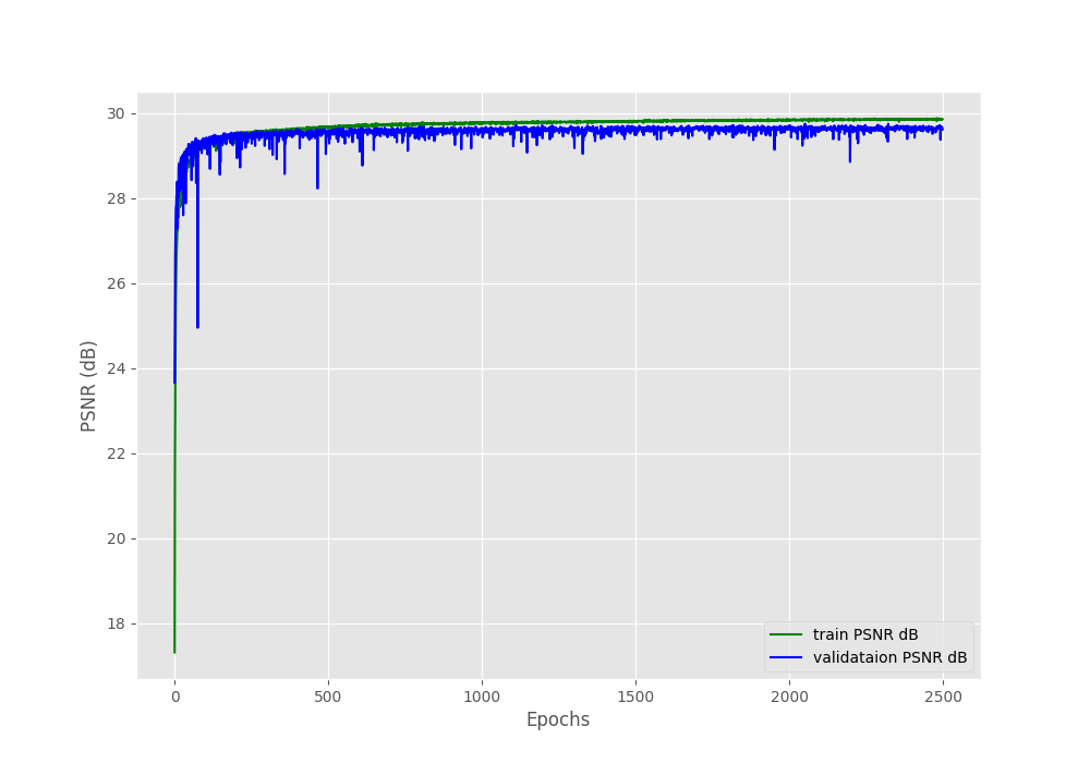
By the end of 2500 epochs, the training PSNR is 29.850 and the validation PSNR is 29.613. Although we cannot directly compare our validation PSNR with that of the paper because we used a combined validation set, still, it is lower than that. This is quite obvious as we have trained for very few iterations compared to the paper. Still, it is a good starting point.

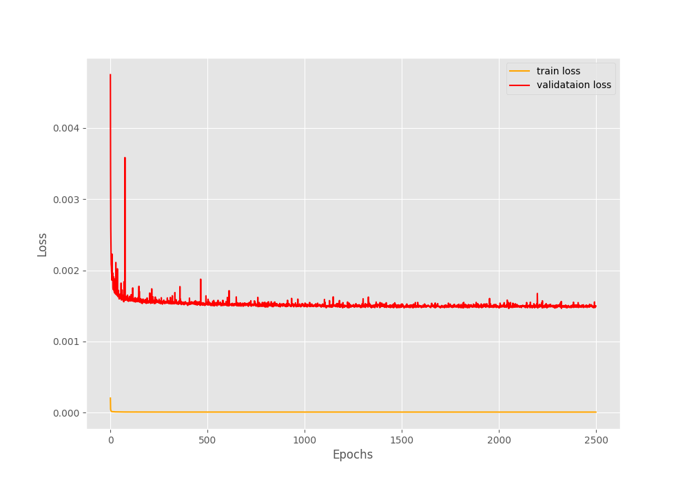
The following are the loss and PSNR graphs.

It is pretty clear that the validation loss remains much higher than the training loss throughout the training. But the important metric here is PSNR. We can see that the training PSNR goes slightly higher than the validation PSNR.

Compare the Validation Reconstruction Images

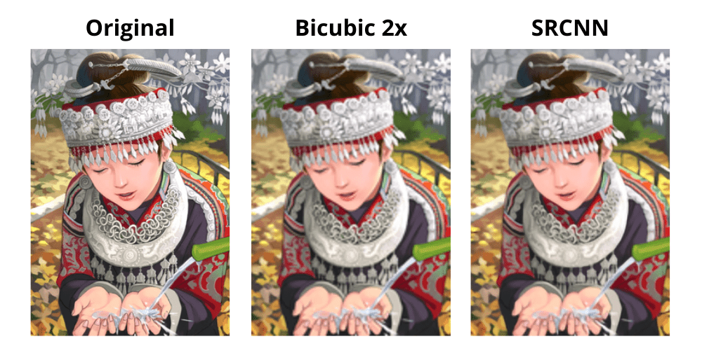
Here are a few comparisons of the validation reconstructed images that are saved to disk. All these validation reconstructed images are from the final epoch.

We can see that although the reconstructed image is not as clear as the real high resolution image, still, it is much better compared to the upscaled bicubic image.

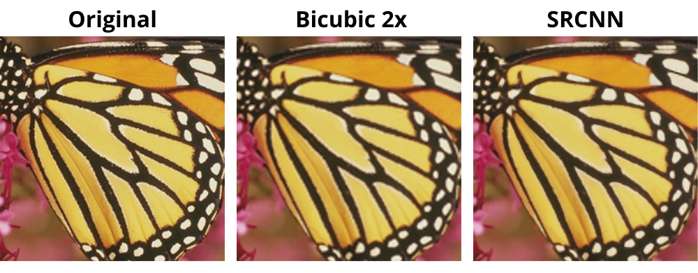
The following is another comparison where the reconstruction is pretty good compared to the bicubic one.

For a final comparison let’s look at one where the improvements are not that apparent.

For sure, the SRCNN results are better, but not that good compared to the previous two results.

Testing on Set5 and Set14 Datasets

For the final part, let’s check out the test PSNR on the Set5 and Set14 datasets. We will not discuss the test script code here. You can find the code in test.py.

Let’s execute it and check out the results.

python test.py

The following are the test results.

100%|██████████████████████████████████████████████████████████████████████| 5/5 [00:00<00:00, 44.18it/s]
Test PSNR on Set5: 32.425
100%|████████████████████████████████████████████████████████████████████| 14/14 [00:00<00:00, 35.00it/s]
Test PSNR on Set14: 28.609

We are getting a test PSNR of 32.425 on the Set5 dataset compared to the 36.65 in the original paper implementation. For the Set14 dataset, our test PSNR is 28.60, whereas it was 32.45 as per the original implementation. As we trained for a very few iterations, so, we could not reach a very high test PSNR. Still, it is a pretty good starting point considering all the things and coding that we covered.

A Few Takeaways and Further Steps for SRCNN Implementation in PyTorch

From the above project, it is pretty clear that training a good model from scratch or implementing a deep learning paper is not that easy when trying to replicate the results. Most of the time, we need a huge amount of computation power. Even if our SRCNN implementation in PyTorch was not able to replicate the results entirely, we learned a lot of things which is at times even more important.

For further experiments, you may combine the T91 dataset with another well know Super Resolution benchmarking dataset, that is, the General100 dataset. This we will be doing in one of the next tutorials and check out even more experimental results on unseen images.

Summary and Conclusion

In this tutorial, we carried SRCNN implementation in PyTorch for Image Super Resolution. We covered the code in detail and also tested our trained model on the Set5 and Set14 datasets. Hopefully, this was a good learning experience for you.

If you have any doubts, thoughts, or suggestions, please leave them in the comment section. I will surely address them.

You can contact me using the Contact section. You can also find me on LinkedIn, and Twitter.