Linear Regression is one of the most simple yet widely used statistical Machine Learning technique. The linear regression machine learning algorithm tries to map one or more independent variable (features) to a dependent variable (scalar output). In this post, you will be learning about:
- Different types of linear regression in machine learning.
- A bit of statistics/mathematics behind it.
- And what kind of problems you can solve with linear regression.
What Exactly is Linear Regression?
Linear Regression is basically a statistical modeling technique. But it is widely used in machine learning as well. In linear regression, we try to predict some output values (y) which are scalar values with the help of some input values (x).
We call the input variables as independent variables as well. This is because these values do not depend on any other values. In the same sense, we call the output scalar values as dependent variables. This is because to find these output scalar values, we depend on the input variables.
Mathematical Representation of Linear Regression
To know the representation of linear regression, we have to consider both the mathematical and machine learning aspects of the problem. But this is going to be really easy to understand, there is nothing fancy about it.
Say, we have a collection of labeled examples,
$${(x_i, y_i)}^N_{i=1}$$
where \(N\) is the size or length of the dataset, \(x_i\) is the feature vector from \(i = 1, …, N\), and \(y_i\) is the real valued target. For more clarity, you can call the collection of \(x_i\) as the independent variables and the collection of \(y_i\) as the dependent or target variables.
I hope that by now you are somewhat clear on how these notations are used in machine learning. If we simplify the above into words, then we can say that:
We want to build a linear model with the combination of features in x and predict the scalar values in y.
When we consider a simple linear regression, that is, a single x and a single y, then we can write,
$$
y = \beta_0 + \beta_1x
$$
where \(\beta_0\) is the intercept parameter and \(\beta_1\) is the slope parameter.
If you analyze the above equation, then you may find that it is the same as the equation of a line:
$$
y = mx + c
$$
where \(m\) is the slope and \(c\) is the y-intercept.
For now, we just need to keep in mind that the above equations are for single-valued x. We will again come back to these to learn how actually they are used in machine learning. First, let’s discuss what is simple linear regression and what is multiple linear regression.
Simple Linear Regression
We know that in linear regression we need to find out the dependent variables (y) by using the independent variables (x).
In simple linear regression, for each observation \(i = 1, 2, …, N\), there is only one \(x_i\) and one \(y_i\). This is the simplest form of linear regression.
For machine learning, a simple linear regression dataset would look something like the following.
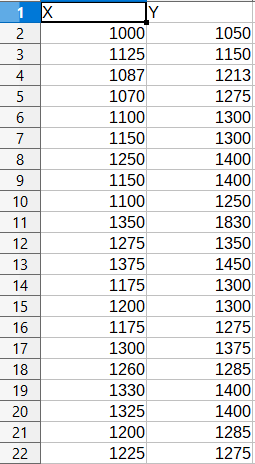
When you analyze the above dataset, then you will see that here, \(N = 22\), and there is one column for the independent variable (X) and one column for the dependent variable (Y). In terms of machine learning, we call the X variables as features and the Y variables as labels or targets.
We have already seen the equation for simple linear regression, that is, \(y = \beta_0 + \beta_1x\).
And we already know that \(\beta_0\) is the intercept parameter and \(\beta_1\) is the slope parameter.
Multiple Linear Regression
In multiple linear regression, we have two or more independent variables (x) and one dependent variable (y). So, instead of a single feature column, we have multiple feature columns and a target column.
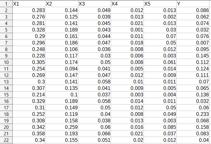
In the above dataset, we have 22 examples, that is \(N = 22\), there are five feature columns and one target column as usual.
How to Use Linear Regression in Machine Learning
In this section, we will see how the mathematical and machine learning concepts merge and how we can predict new output values given some prior data.
Before moving further, you just have to keep a few things in mind.
We have a collection of labeled examples, \({(x_i, y_i)}^N_{i=1}\), where \(x_i\) is the training variable and \(y_i\) is the target variable. Let’s say for \(i = 1, 2, …, 10\) the \(x_i\) values look something like the following on a 2D axis.
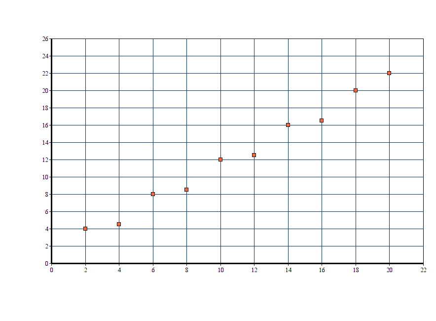
Now, we have to predict some target variable \(y_{new}\) for some give input feature \(x_{new}\). And we know that the equation of a line is given by \(y = mx + c\). Let’s say we get the following line.
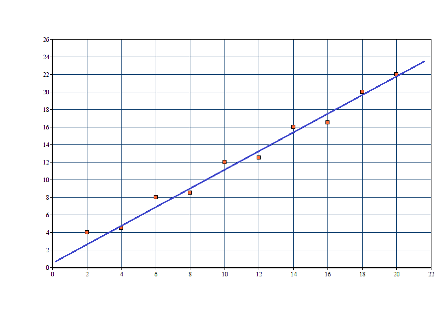
Obviously, we would want the training example (the orange squares) to be as close to the regression line as possible. But how can we do that? We have to find the right values for the parameters \(m\) and \(b\). Then only we will find a good linear model that will predict new values correctly for some given inputs.
To find the right values for the slope and intercept parameters, we use an objective function or more popularly known as a cost function in machine learning. MSE (Mean Squared Error) is one such cost function that is widely used in linear regression.
Mean Squared Error Cost Function
In this section, we will cover the MSE cost function and see how it is used in linear regression.
MSE is the average squared difference between the \(y_i\) values that we have from the labeled set and the predicted \(y_{new}\) values. We have to minimize this average squared difference to get a good regression model on the given data.
The following is the formula for MSE:
$$
MSE = \frac{1}{N}\sum{(y_i – (mx_i + b))}^2
$$
In the above equation, \(N\) is the number of labeled examples in the training dataset, \(y_i\) is the target value in the dataset and \((mx_i + b)\) is the predicted value of the target or you can say \(y_{new}\).
Minimizing the above cost function will mean finding the new target values as close as possible to the training target values. This will ensure that the linear model that we find will also lie close to the training examples.
To minimize the above cost function, we have to find the optimized values for the two parameters \(m\) and \(b\). For that, we use the Gradient Descent method to find the partial derivatives with respect to \(m\) and \(b\). In that case, the cost function looks something like the following:
$$
f(m,b) = \frac{1}{N} \sum_{i=1}^{n} (y_i – (mx_i + b))^2
$$
Next, we use the chain rule to find the partial derivative of the above function. To solve the problem, we move through the data using updated values of slope and intercept and try to reduce the cost function as we do so. This part is purely mathematical and the machine learning implementation is obviously through coding.
Problem Solving using Linear Regression
Although linear regression models are one of the oldest statistical learning techniques, they are still used in solving a number of real-world problems. Every time, we do not need a very complex learning model to find the right fit for the data in hand. If the problem is simple, then applying a complex learning algorithm may lead to overfitting. We obviously do not want that.
Predicting the increase in sales due to the increase in advertisement budget is one such example where linear regression can be used.
Predicting the increase in call duration for a telephone company after introducing new offers can also be solved using linear regression.
If you want, then you can collect linear regression datasets online and practice to improve your machine learning skills. Kaggle is a great place to get your hands on some amazing datasets. Also, consider using Scikit-Learn library which has almost any machine learning algorithm implementation you can think of.
Summary and Conclusion
In this article, you learned how linear regression works in machine learning and how the mathematical and machine learning concepts merge.
For further reading, you can take a look at the following resources.
Online resources:
1. Wikipedia
2. Linear Regression – ML Cheat Sheet
3. Ordinary Least Squares Regression
Books:
1. The Hundred Page Machine Learning Book
Subscribe to the website to get regular quality posts right into your inbox. You can follow me Twitter and LinkedIn as well to get regular updates.



1 thought on “Linear Regression in Machine Learning”