Introduction to BiRefNet

In recent years, the need for high-resolution segmentation has increased. Starting from photo editing apps to medical image segmentation, the real-life use cases are non-trivial and important. In such cases, the quality of dichotomous segmentation maps is a necessity. The BiRefNet segmentation model solves exactly this. In this article, we will cover an introduction to BiRefNet and how we can use it for high-resolution dichotomous segmentation.

The dichotomous image segmentation task aims at dividing an image into two distinct regions, namely, foreground (the object of interest) and background. In recent years, many deep learning models have been proposed for this task. However, the BiRefNet model is one that stands out because of is methodology and architecture.

What will we cover in the introduction to BiRefNet?

• What is BiRefNet?
• What is its architecture, and why does it stand out?
• How does BiRefNet learn so effectively?
• How does its performance compare to other models?
• Which datasets has BiRefNet been trained on?
• What real-life use cases can we use BiRefNet for?
• How to run a simple background removal task using BiRefNet?

What is BiRefNet?

BiRefNet, short for Bilateral Reference Network, is a novel deep learning framework designed specifically for high-resolution dichotomous image segmentation.

It was introduced in the paper Bilateral Reference for High-Resolution Dichotomous Image Segmentation by Zhen et al.

Its primary goal is to produce segmentation masks of exceptional quality, capturing the finest details that other models often miss. For example, the individual strands of hair on a person’s head or the intricate patterns on a delicate object.

Previous models often struggled with a fundamental trade-off: to understand the overall context of an image (what the object is). Furthermore, they had to downsize the image, which inevitably leads to the loss of fine details. BiRefNet introduces a clever architecture to overcome this, allowing it to “see” both the big picture and the tiny pixels simultaneously.

What Is Its Architecture, and Why Does It Stand Out?

The architecture of BiRefNet is what sets it apart. It smartly decomposes the segmentation task into two main modules: a Localization Module (LM) and a Reconstruction Module (RM).

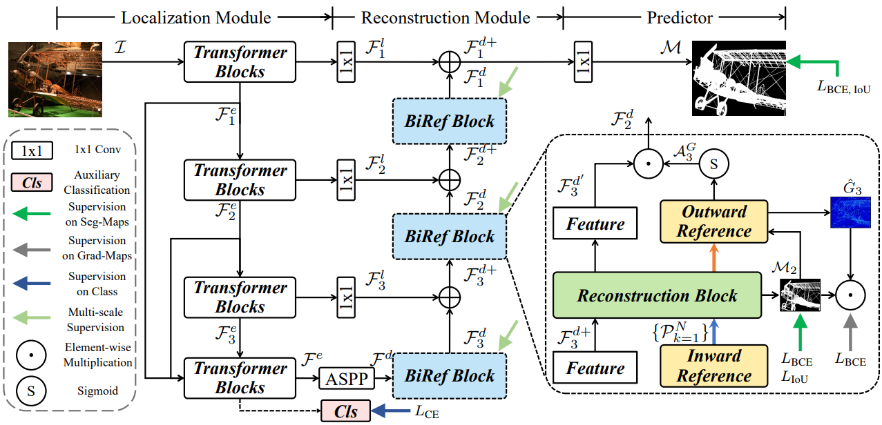
Localization Module (LM): Identifying the Target

This module’s job is to first figure out the general location and coarse shape of the target object. It uses a Swin Transformer as its backbone to analyze the image and produce a low-resolution “rough draft” of the segmentation. To improve its understanding of the image content, the LM also includes an auxiliary classification head, which helps it learn a better semantic representation of the object.

Reconstruction Module (RM) with Bilateral Reference: Perfecting the Details

The RM takes the output from the LM and refines it into a high-precision, final mask. To do this, it uses a unique mechanism called Bilateral Reference (BiRef). This provides information from two crucial sources.

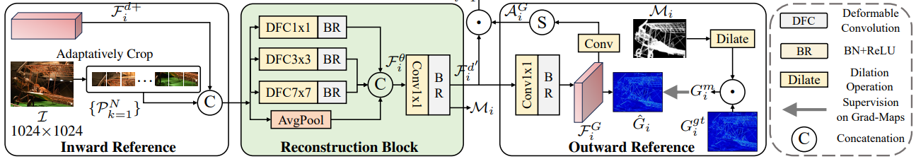
• Inward Reference (Source Image Guidance): Instead of working with a downscaled, blurry version of the image, the RM directly references the original, full-resolution image. At every stage of the decoding process, it adaptively crops patches from the original image that correspond to the feature map’s location. This ensures that the fine textures, sharp edges, and intricate details are not lost and can be used to create a highly accurate boundary. The features are then processed using deformable convolutions, which are excellent at handling objects with complex shapes.
• Outward Reference (Gradient Supervision): To guide the model’s focus, the authors also train the RM using gradient maps. It highlights all the edges and high-detail areas of an object. It forces the model to learn to pay special attention to these complex regions. The model also uses a masking strategy to ensure it focuses only on the gradients of the target object.

This dual-reference approach is the secret to BiRefNet’s success. It allows the model to leverage global context from the LM. All the while, reconstructing details using direct references to the original image.

How BiRefNet Learns?

The training methodology is equally crucial for achieving state-of-the-art results.

Smart Training Strategies

Training on high-resolution images is computationally expensive. The BiRefNet paper outlines several practical strategies to maximize performance and efficiency:

• Multi-Stage Supervision (MSS): The authors apply supervision at multiple stages of the decoder. This acts as a shortcut for the learning process. It accelerates convergence and allows the model to achieve top performance in fewer training epochs (e.g., 200 instead of 400).
• Region-Level Fine-tuning: In the final stages of training, the fine-tuning happens using a loss function that focuses on region-level accuracy (like IoU loss). This helps to further refine the predicted masks and improve metrics. This aligns more with practical applications.

A Hybrid Loss Function

BiRefNet uses a hybrid loss function that combines four different objectives:

• Binary Cross-Entropy (BCE) Loss: For accurate pixel-level classification.
• Intersection over Union (IoU) Loss: To ensure the overall shape and region of the mask are correct.
• Structural Similarity (SSIM) Loss: To preserve the fine structural details and boundaries of the object.
• Cross-Entropy (CE) Loss: For the auxiliary classification task in the Localization Module.

This allows the model to learn to produce masks that are not only pixel-perfect but also structurally coherent.

How Does Its Performance Compare to Other Models?

Let’s discuss some of the important benchmark results from the paper.

Quantitative Results

Across all major datasets for dichotomous segmentation (DIS5K), salient object detection (HRSOD), and concealed object detection (COD), BiRefNet consistently sets a new state of the art. It shows significant improvements in multiple metrics:

• S-measure (Sm): Measures structural similarity. BiRefNet improves this by up to 5.6% on COD benchmarks.
• F-measure (Fβ): A weighted score of precision and recall, where BiRefNet also leads.
• Human Correction Efforts (HCE): A metric that estimates how many clicks a user would need to fix the mask. BiRefNet achieves a lower (better) HCE score, indicating its predictions are closer to a perfect result.

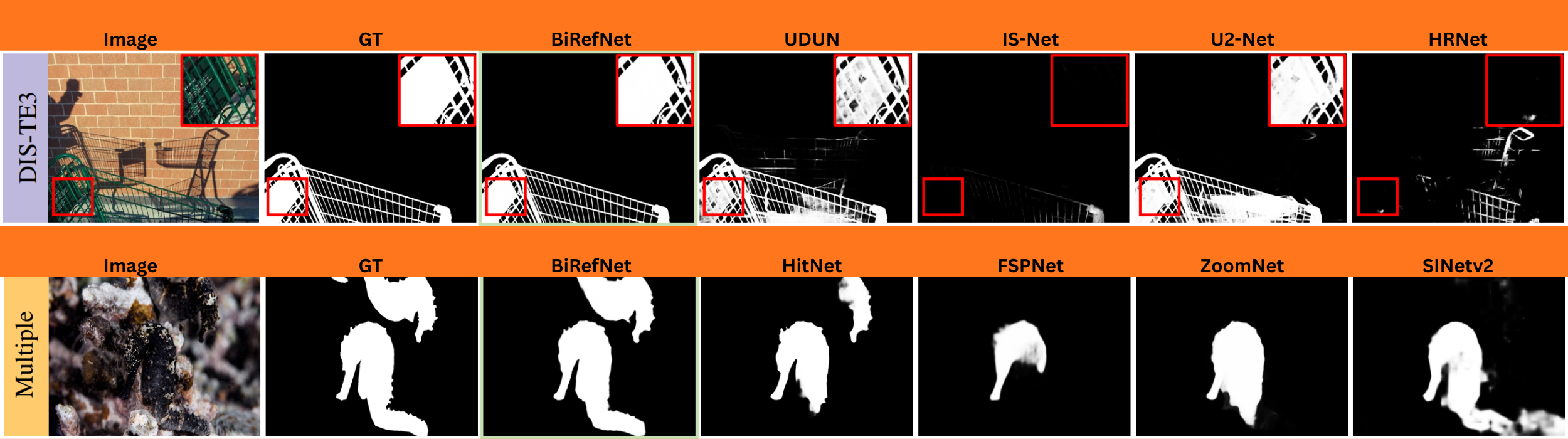
Qualitative Results

When compared side-by-side with other models, BiRefNet demonstrates a clear superiority in handling difficult cases:

• Fine Structures: It flawlessly segments extremely thin objects like bicycle spokes, plant stems, and fences, which other models often miss entirely.
• Complex Textures: It accurately captures intricate details like hair, fur, and complex patterns without over-smoothing.
• Occluded and Slim Objects: It can correctly identify and segment objects that are partially hidden or have very slender parts.

Which Datasets Has BiRefNet Been Trained On?

BiRefNet was trained on datasets specifically curated for high-resolution segmentation.

Its primary training dataset is DIS5K. It is the benchmark for Dichotomous Image Segmentation. This dataset contains thousands of high-resolution images with complex objects, making it ideal for training a model to handle fine details. To prove its versatility, the authors also train and test BiRefNet on benchmarks for other related tasks, including HRSOD and COD, demonstrating its robustness.

What Real-Life Use Cases Can We Use BiRefNet For?

The high-quality segmentation maps produced by BiRefNet have numerous practical and creative applications.

• Professional Photo and Video Editing: The most direct application is flawless background removal. BiRefNet can separate a subject from its background, which is invaluable for e-commerce product images, marketing materials, and professional graphic design.
• Creative AI and Generative Art: BiRefNet has already been embraced by the AI art community. ComfyUI (for Stable Diffusion) uses it in workflows to create perfect masks. Artists can use these masks to seamlessly change backgrounds, apply targeted effects, or guide generative models to modify only specific parts of an image with incredible precision.
• Industrial and Architectural Inspection: We can use BiRefNet for automated inspection. For example, we can train it to detect tiny cracks in building facades, bridges, or industrial equipment from photographs, helping to identify structural issues early.
• Rapid Community Adoption: A testament to its utility, BiRefNet has seen rapid adoption. Developers have created online demos (e.g., on Fal.AI) and integrated it into user-friendly tools, making this powerful technology accessible to a broader audience beyond researchers.

In the next section, we will start creating a small background removal codebase using BiRefNet.

Background Removal Using BiRefNet

Before we move to the coding part, make sure to clone the BiRefNet GitHub repository.

Cloning the BiRefNet Repository

git clone https://github.com/ZhengPeng7/BiRefNet.git

This includes all the modules related to models, filtering out backgrounds, and creating alpha channel subject masks.

Final Project Directory Structure

Let’s take a look at the final project directory structure.

├── backgrounds
│   ├── bg_1.jpg
│   └── bg_2.jpg
├── evaluation
│   └── metrics.py
├── images
│   ├── image_1.jpg
│   ├── image_2.jpg
│   └── image_3.jpg
├── models
│   ├── backbones
│   ├── modules
│   ├── refinement
│   └── birefnet.py
├── predictions
│   ├── image_3-mask.png
│   └── image_3-subject.png
├── tutorials
│   ├── BiRefNet_inference.ipynb
│   ├── BiRefNet_inference_video.ipynb
│   └── BiRefNet_pth2onnx.ipynb
├── bg_removal_inference.ipynb
├── BiRefNet-general-epoch_244.pth
├── config.py
├── dataset.py
├── eval_existingOnes.py
├── gen_best_ep.py
├── image_proc.py
├── inference.py
├── LICENSE
├── loss.py
├── make_a_copy.sh
├── README.md
├── requirements.txt
├── rm_cache.sh
├── sub.sh
├── test.sh
├── train.py
├── train.sh
├── train_test.sh
└── utils.py

• We will focus on the bg_removal_inference.ipynb Jupyter Notebook, which contains all the code that we need for background removal using BiRefNet.
• We have some additional folders as well. images contains all the images that we will run segmentation and background removal on. predictions contains the results from BiRefNet segmentation results.
• The BiRefNet-general-epoch_244.pth is the model weight file that will be downloaded via the Jupyter Notebook.

Other than the Jupyter Notebook and the images directory, all other files and folders are part of the repository.

You can install the requirements using the requirements.txt file.

pip install -r requirements.txt

The Jupyter Notebook and inference images are available to download via the download section. After downloading, keep them in the cloned BiRefNet directory.

Download Code

Import Statements Required for Background Removal

Let’s jump into the code now. All the code that we will go through here is present in the bg_removal_inference.ipynb notebook.

We will start with downloading the weights and the necessary import statements.

!wget https://github.com/ZhengPeng7/BiRefNet/releases/download/v1/BiRefNet-general-epoch_244.pth

We are downloading the BiRefNet General model that has been pretrained for 244 epochs.

import torch
import os
import cv2
import matplotlib.pyplot as plt
import numpy as np

from PIL import Image
from torchvision import transforms
from IPython.display import display
from models.birefnet import BiRefNet
from utils import check_state_dict
from glob import glob
from image_proc import refine_foreground

The above import statements contain all the modules that we will need further.

• From the models module of BiRefNet, we are importing the BiRefNet class.
• We also import a refine_foreground function from image_proc module that we will use to create the masked image.

Next, we define the computation device.

device = torch.device('cuda') if torch.cuda.is_available() else torch.device('cpu')

It is best to run the notebook on a CUDA device, as I have encountered issues with CPU. On CPU devices, the inference might go on indefinitely without finishing. Although I am yet to debug deeper into that.

Load the BiRefNet Model

The next function loads the BiRefNet model.

def load_model(model_name='BiRefNet'):
    """
    Choose from: 'BiRefNet', 'BiRefNet_HR', 'BiRefNet_HR-matting'
    """

    birefnet = BiRefNet(bb_pretrained=False)
    state_dict = torch.load('BiRefNet-general-epoch_244.pth', map_location=device)
    state_dict = check_state_dict(state_dict)
    birefnet.load_state_dict(state_dict)
    
    # Load Model
    torch.set_float32_matmul_precision(['high', 'highest'][0])
    
    birefnet.to(device)
    birefnet.eval()
    print('BiRefNet is ready to use.')
    birefnet.half()

    return birefnet

First, the function loads the weight files onto the computation device and then loads the weights into the model.

We return the model in FP16 format.

The next block of code defines the model name we are going to use and the transforms that are needed.

# Choose from: 'BiRefNet', 'BiRefNet_HR', 'BiRefNet_HR-matting'
model_name = 'BiRefNet_HR'
model = load_model(model_name)

transform_image = transforms.Compose([
    transforms.Resize((1024, 1024) if '_HR' not in model_name else (2048, 2048)),
    transforms.ToTensor(),
    transforms.Normalize([0.485, 0.456, 0.406], [0.229, 0.224, 0.225])
])

If we choose to use an HR (High-Resolution) format, then the transforms will resize the images to 2048×2048 resolution. Else, they will be resized to 1024×1024 resolution. This also affects the final segmentation map and the GPU memory needed.

For non-high-resolution workflows, the GPU requirement is around 5.5GB, whereas for high-resolution inference, around 9.5GB of VRAM is needed.

Function to Remove Background

The following code block contains the logic to remove the background and separate the foreground (object of interest).

def run_inference(image_path):
    image = Image.open(image_path)
    input_images = transform_image(image).unsqueeze(0).to(device)
    input_images = input_images.half()

    # Prediction
    with torch.no_grad():
        preds = model(input_images)[-1].sigmoid().cpu()
    pred = preds[0].squeeze()

    # Save Results
    file_ext = os.path.splitext(image_path)[-1]
    pred_pil = transforms.ToPILImage()(pred)
    pred_pil = pred_pil.resize(image.size)
    pred_pil.save(image_path.replace(src_dir, dst_dir).replace(file_ext, '-mask.png'))
    image_masked = refine_foreground(image, pred_pil)
    image_masked.putalpha(pred_pil)
    image_masked.save(image_path.replace(src_dir, dst_dir).replace(file_ext, '-subject.png'))

    # Visualize the last sample:
    # Scale proportionally with max length to 1024 for faster showing
    scale_ratio = 1024 / max(image.size)
    scaled_size = (int(image.size[0] * scale_ratio), int(image.size[1] * scale_ratio))
    
    display(image_masked.resize(scaled_size))
    display(image.resize(scaled_size))
    display(pred_pil.resize(scaled_size))

The function accepts an image path, reads it using PIL, and carries out the forward pass.

After we get the predictions (preds), which is simply a binary mask, we get the masked image also. This masked image is an alpha channel image which contains the foreground object.

The next code block runs the inference and saves the results in the predictions directory.

src_dir = 'images'
image_paths = glob(os.path.join(src_dir, '*'))
dst_dir = 'predictions'
os.makedirs(dst_dir, exist_ok=True)

for image_path in image_paths:
    print('Processing {} ...'.format(image_path))
    run_inference(image_path)
    # break

Analyzing the Results

Let’s take a look at the three results from the images.

The results are quite fascinating. The segmentation maps of the jellyfish and the woman are quite detailed. Even the finer lines are properly segmented.

However, in the case of the bicycle, the spokes appear to be a bit distorted. This is perhaps because the background (water) matches the color of the spokes, and the model was unable to segment them properly. Still, these are impressive results.

In the next article, we will focus on creating a simple background replacement app using BiRefNet.

Summary and Conclusion

In this article, we focused on a simple introduction to BiRefNet. Along with discussing the important bits from the paper, we also ran inference for background removal using BiRefNet.

If you have any questions, thoughts, or suggestions, please leave them in the comment section. I will surely address them.

You can contact me using the Contact section. You can also find me on LinkedIn, and X.

References

• Bilateral Reference for High-Resolution Dichotomous Image Segmentation
• BiRefNet GitHub