Linear Regression is one of the oldest statistical learning methods that is still used in Machine Learning. Also, it is quite easy for beginners in machine learning to get a grasp on the linear regression learning technique. In this article, we will be implementing Simple Linear Regression from Scratch using Python.
Note: If you want to get a bit more familiarity with Linear Regression, then you can go through this article first. It will teach you all the basics, including the mathematics behind linear regression, and how it is actually used in machine learning.
The Linear Regression Equation
Before diving into the coding details, first, let’s know a bit more about simple linear regression.
In simple linear regression, we have only one feature variable and one target variable. Let the feature variable be x and the output variable be y. Our job is to find the value of a new y when we have the value of a new x.
The equation for the above operation is,
$$
y = \beta_0 + \beta_1x
$$
where \(\beta_0\) is the intercept parameter and \(\beta_1\) is the slope parameter.
So, we will have to build a linear model by using the features x and target y that should be a straight line plot on a graph. For that, we have to optimize the parameters \(\beta_0\) and \(\beta_1\) using a cost function (also known as objective function).
So, fire up your favorite IDE or Jupyter Notebook and follow along.
Using Scikit-Learn Make Regression
As this post is meant to be an introductory one, so we will be using Scikit-Learn’s make_regression module to generate random regression data.
Let’s get our data from Scikit-Learn first.
import numpy as np
import matplotlib.pyplot as plt

from sklearn.datasets import make_regression
x, y = make_regression(n_samples=200, n_features=1, noise=20, bias=0)
Now, we have 1 feature and 200 sample values in total. x holds all the feature values and y holds all the target values.
def plot_fig(x, y, b0, b1, name):
    plt.figure()

    plot_x = np.linspace(min(x), max(x), 200)
    plot_y = b0 + b1 * plot_x

    plt.scatter(x, y)

    plt.plot(plot_x, plot_y, color='red')

    plt.savefig(name)
The above function defines the scatter plot for the feature values and their corresponding targets. It will also plot our linear model when we give it the slope and intercept parameters. It takes four arguments, the data points x, the targets y, and both of the simple linear regression parameters.
Initial Plotting
We do not have any optimal values for b0 and b1 till now. We need to optimize both these values so that we will have the best fit for the data in hand.
We can randomly initialize the values for b0 and b1 so that we can visualize the initial linear model before any optimization. Later we will be optimizing the values to get the best linear model that we can. The code snippet below initializes the parameters b0 and b1 with random values.
b0= np.random.rand()
b1 = np.random.rand()
Now, to visualize the initial linear model and the data points, let’s call the plot_fig() function.
plot_fig(x, y, b0, b1)
The above code gives us the following plot as output:
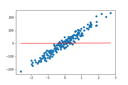
We can clearly see that the linear regression line is not at all a good fit, at least for now. Let’s move ahead and try to get better results.
Define the Cost Function
In almost all types of learning, to make the algorithm learn from data, we need to minimize some sort of cost function. This cost function is otherwise known as an objective function. In the case of linear regression, we are going to optimize the Mean Square Error (MSE). The following is the mathematical expression of MSE.
$$
MSE = \frac{1}{N} \sum_{i=1}^{n} (y_i – (m x_i + b))^2
$$
By using the above function we will optimize the slope and intercept parameters. In some books and articles, you may encounter the word ‘weight’ for the slope (\(m\)) parameter and ‘bias’ for the intercept parameter (\(m\) ). This is a common practice in machine learning terms.
So, what do we do to minimize the cost function? We use the Gradient Descent method. As we have to optimize both the parameters, we will have to use partial derivative for that. Also, the cost functions will be dependent on two parameters now.
$$
f(m,b) = \frac{1}{N} \sum_{i=1}^{n} (y_i – (mx_i + b))^2
$$
To get into the mathematical aspects, you see refer to this amazing article.
We are now ready to define the code for implementing the cost function. The following code block does so.
# cost function
def cost_function(x, y, b1, b0):
    num_values = len(x)
    total_error = 0.0
    for i in range(num_values):
        total_error += (y[i] - (b1*x[i] + b0))**2
    return total_error / num_values
Update the Weights
Okay, to optimize the parameters, we need to update them, and use those updated values in each iteration. In the next function, we will update the weights. But first, we calculate the partial derivatives. Then we need to update b0 and b1. We will do so by subtracting the partial derivative values from b0 and b1.
def update_weights(x, y, b1, b0, learning_rate):
    b1_deriv = 0
    b0_deriv = 0
    num_values = len(x)

    for i in range(num_values):
        # Calculate partial derivatives
        b1_deriv += -2*x[i] * (y[i] - (b1*x[i] + b0))

        b0_deriv += -2*(y[i] - (b1*x[i] + b0))

    # update the weights
    b1 -= (b1_deriv / num_values) * learning_rate
    b0 -= (b0_deriv / num_values) * learning_rate

    return b1, b0
update_weights() function accepts five arguments. We pass the data points x and targets y as usual along with b0 and b1. The fifth argument is the learning rate. Learning rate specifies how quickly our algorithm will converge to an optimal solution (find a solution).
Learning rate is a very important parameter. We do not want it to be too high, as it may miss the optimal solution because of very large steps. We also do not want it to be too low. In that case, the steps will be more and the convergence may take a lot of time to happen.
The Training Function
Finally, we define the function to train the algorithm. In addition to the five arguments that update_weights() function accepts, it takes one more argument. That is the number of iterations. The number of iterations defines how many times our algorithms will be trained on the data fully. For a low learning rate, number iterations will be high and for a high learning rate, it will be less.
def train(x, y, b1, b0, learning_rate, iterations):
    costs = []

    for i in range(iterations):
        b1, b0 = update_weights(x, y, b1, b0, learning_rate)

        # calculate the cost
        cost = cost_function(x, y, b1, b0)
        costs.append(cost)

        # plot the linear model
        if i % 50 == 0:
            plot_fig(x, y, b0, b1, name='linear-epoch-'+str(i))

    return b1, b0, costs
In the end, we just call the train() function. We will run the algorithm for 200 epochs and plot the linear model every 50 epochs to get a good look at the learning process. Also, the learning rate is going to be 0.01.
train(x, y, b1, b0, 0.01, 200)
We get four plots for the linear model while training process. The following four are those plots.
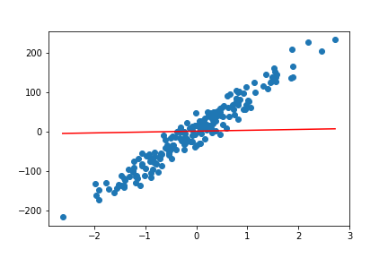
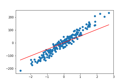
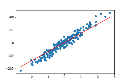

By the end of 200 epochs our model seems to do pretty well. You can always try to play around with different learning rates and epochs. This will give you better insights on how these affect the linear regression model.
Summary and Conclusion
In this article, you learned how to implement simple linear regression from scratch. Obviously, you do not need to write such code while doing practical industry-oriented machine learning. There are amazing libraries like Scikit-Learn which help us to carry these out with much ease.
Subscribe to the website to get timely article information in your inbox. You can also follow me Twitter and LinkedIn to get regular updates about my articles.

