
In this article, we will be fine tuning the LRASPP MobileNetV3 model on the KITTI segmentation dataset.
This article is the first in the series where we fine-tune the LRASPP MobileNetV3 model for Autonomous Driving Scene Segmentation. For this, we will start with fine-tuning the model on the KITTI semantic segmentation dataset. This is a small dataset that will kickstart our experiments. We will try two different training approaches and figure out how well the model can segment complex driving scenes. In the next two articles, we will use larger segmentation datasets for fine tuning to produce better models and optimize them for CPU inference & lower latency.
We will cover the following components in this article
- We will start with a discussion of the KITTI segmentation dataset.
- Next, we will discuss the directory structure of the entire project.
- We will follow this with our training experiments of the LRASPP MobileNetV3 model. This includes:
- Fine tuning the LRASPP MobileNetV3 model on the original images.
- Fine tuning the model on a larger set where we split each image of the KITTI dataset into two halves.
- Next, we will run inference using the best trained models.
The KITTI Segmentation Dataset
The KITTI dataset contains images from driving scenes in real-world scenarios. The dataset that we are going to use is available here on Kaggle.
It is a small experimental dataset containing just 203 images spanning over 14 classes.
- ‘car’,
- ‘road’,
- ‘mark’,
- ‘building’,
- ‘sidewalk’,
- ‘tree’,
- ‘pole’,
- ‘sign’,
- ‘person’,
- ‘wall’,
- ‘sky’,
- ‘curb’,
- ‘grass’,
- ‘void’
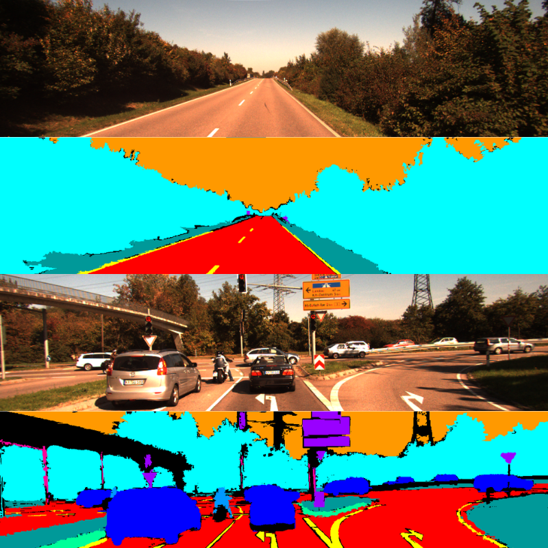
Here are a few images along with their ground truth segmentation masks.
Each image is 1241 pixels in width and 376 pixels in height. Downloading the dataset will reveal the following directory structure.
├── calibrations
├── images
├── labels
├── labels_new
├── match_file.txt
├── README.html
├── README.md
├── rwth_kitti_semantics_dataset
└── splits
The images directory contains RGB images and the labels directory the segmentation maps. The splits directory contains the train.txt and test.txt files with the names of the samples to use for training and testing. We will use these files later to create the splits before training.
Project Directory Structure
Following is the directory structure for the entire project.
├── input
│   ├── calibrations
│   ├── images
│   ├── inference_data
│   ├── labels
│   ├── labels_new
│   ├── rwth_kitti_semantics_dataset
│   ├── split_data
│   ├── split_data_half
│   ├── splits
│   ├── match_file.txt
│   ├── README.html
│   └── README.md
├── outputs
│   ├── normal_training
│   └── split_training
├── src
│   ├── __pycache__
│   ├── config.py
│   ├── create_data_folder_half_image.py
│   ├── create_data_folders.py
│   ├── datasets.py
│   ├── engine.py
│   ├── inference_image.py
│   ├── inference_video.py
│   ├── metrics.py
│   ├── model.py
│   ├── train.py
│   └── utils.py
└── requirements.txt
- The
srcdirectory contains all the Python code files. - In the
outputsfolder, we have the results from the training and inference experiments. - The
inputdirectory contains the KITTI segmentation dataset. Along with that, it contains two additional directories,split_dataandsplit_data_half. We will create these two data directories before starting the training experiments. - The project directory also contains the
requirements.txtfile to install the major requirements.
All the trained weights and the source code files will be available via the download section. If you wish to train the model, you need arrange the dataset in the above structure.
Download Code
Installing the Dependencies
The source code uses PyTorch 2.0.1. It is recommended to use the Anaconda package manager and install the PyTorch version using the following command.
conda install pytorch==2.0.1 torchvision==0.15.2 torchaudio==2.0.2 pytorch-cuda=11.8 -c pytorch -c nvidia
Furthermore, you can install the rest of the requirements via the requirements file.
pip install -r requirements.txt
This is all the setup we need for following along with this article.
Fine Tuning LRASPP MobileNetV3 on the KITTI Segmentation Dataset
Let’s move to the coding part now. As the codebase is quite extensive, we will not go through all the Python files. We will only go through some of the necessary ones. However, as they are available for download, feel free to explore them before moving forward.
The LRASPP MobileNetV3 Semantic Segmentation Model
As of writing this, the LRASPP MobileNetV3 is the smallest and most efficient pretrained semantic segmentation model available in the Torchvision library. It has around 3.2 million parameters and can run in almost real-time even on an older GTX 1060 laptop GPU.
If you wish to know more about the pretrained model performance, check out the article where we run inference using the LRASPP MobileNetV3 segmentation model.
The code for loading the model is present in the model.py file. Here is the entire file content.
import torch.nn as nn

from torchvision.models.segmentation import lraspp_mobilenet_v3_large

def prepare_model(num_classes=2):
    model = lraspp_mobilenet_v3_large(weights='DEFAULT')
    model.classifier.low_classifier = nn.Conv2d(
        40, num_classes, kernel_size=(1, 1), stride=(1, 1)
    )
    model.classifier.high_classifier = nn.Conv2d(
        128, num_classes, kernel_size=(1, 1), stride=(1, 1)
    )
    return model

if __name__ == '__main__':
    model = lraspp_mobilenet_v3_large(weights='DEFAULT')

    print(model)
    # Total parameters and trainable parameters.
    total_params = sum(p.numel() for p in model.parameters())
    print(f"{total_params:,} total parameters.")
    total_trainable_params = sum(
        p.numel() for p in model.parameters() if p.requires_grad)
    print(f"{total_trainable_params:,} training parameters.")
After loading the model from Torchvision, we modify the number of classes in the final classifier layers to match the number of classes in our dataset. By default, it has been pretrained on images from COCO using the 20 categories from the Pascal VOC dataset.
Preparing the Dataset for Training on the Original Dataset
The original dataset has the images and labels in a single directory. We will prepare a simple script that will divide the samples into a training and validation set based on the split text files. Following is the code that is present in the create_data_folders.py file.
import os
import shutil

from tqdm.auto import tqdm

splits = ['train', 'val']
DST_DIR = '../input/split_data'
IMG_DIR = os.path.join(DST_DIR, 'images')
LBL_DIR = os.path.join(DST_DIR, 'labels')

ROOT_IMG_DIR = '../input/images'
ROOT_LBL_DIR = '../input/labels'

os.makedirs(DST_DIR, exist_ok=True)
for split in splits:
    os.makedirs(os.path.join(IMG_DIR, split), exist_ok=True)
for split in splits:
    os.makedirs(os.path.join(LBL_DIR, split), exist_ok=True)

train_file = open('../input/splits/train.txt', 'r')
train_images = train_file.readlines()
train_images = [train_image.rstrip().split('images/')[-1] for train_image in train_images]
print(train_images)

test_file = open('../input/splits/test.txt', 'r')
test_images = test_file.readlines()
test_images = [test_image.rstrip().split('images/')[-1] for test_image in test_images]
print(test_images)

# Copy data to respective directories.
def copy(split='train', data_list=None):
    for data in tqdm(data_list, total=len(data_list)):
        data_name = data.split('.pcd')[0]
        image_path = os.path.join(ROOT_IMG_DIR, data_name+'.png')
        label_path = os.path.join(ROOT_LBL_DIR, data_name+'.png')

        shutil.copy(
            image_path,
            os.path.join(IMG_DIR, split, data_name+'.png')
        )
        shutil.copy(
            label_path,
            os.path.join(LBL_DIR, split, data_name+'.png')
        )

copy(split='train', data_list=train_images)
copy(split='val', data_list=test_images)
We can run this script from within the src directory by executing the following command.
python create_data_folders.py
This will create the split_data folder within the input directory that we saw while going through the project structure. The images and labels will have their subdirectories for the training and validation sets. In the end, we have 120 training samples and 83 validation samples.
Fine Tuning the LRASPP MobileNetV3 Segmentation Model using the Original Images
Now we can run training using the original images.
All the training experiments shown in this article were run on a system with a 10 GB RTX 3080 GPU, 10th generation i7 CPU, and 32 GB of RAM.
We can execute the train.py script with the necessary command line arguments to start the training.
python train.py --batch 8 --height 376 --width 1240 --lr 0.05 --epochs 100 --out normal_training --data ../input/split_data
Here are all the arguments that we use:
--batch: The batch size for preparing the data loaders.--heightand--width: The height and width of the images to resize while preprocessing the images. We keep the same dimensions as the original images.--lr: Learning rate for the optimizer. We are using a higher learning rate of 0.05 as this worked for this training experiment.--epochs: The number of epochs to train for. We are training for 100 epochs here.--out: The path to the output directory. This will create a subdirectory within theoutputsdirectory with the name that we provide here. It becomes easier to differentiate between experiments this way.--data: Finally, the path to the input data for training.
The model reached the best Mean IoU on the last epoch. Here are the logs from the final epoch.
EPOCH: 100
Training
100%|████████████████████| 15/15 [00:03<00:00,  3.85it/s]
Validating
100%|████████████████████| 11/11 [00:02<00:00,  4.58it/s]

Best validation IoU: 0.31890310503549935

Saving best model for epoch: 100

Train Epoch Loss: 0.4093, Train Epoch PixAcc: 0.8114, Train Epoch mIOU: 0.424317
Valid Epoch Loss: 0.6861, Valid Epoch PixAcc: 0.7304 Valid Epoch mIOU: 0.318903
--------------------------------------------------
TRAINING COMPLETE
We have the best model trained on the original images with a Mean IoU of 31.89%.
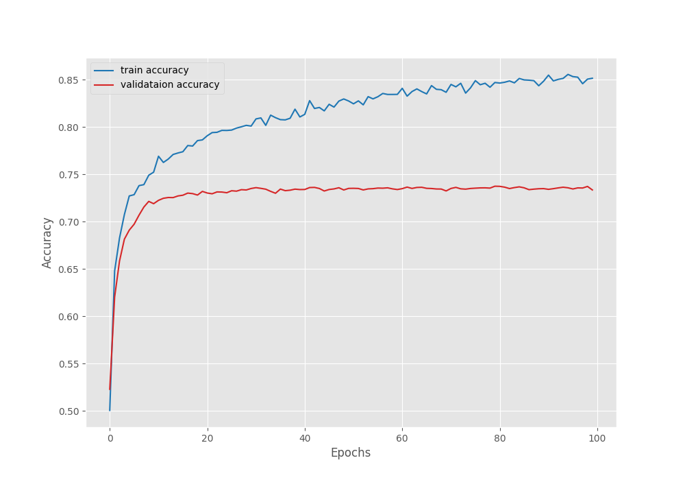
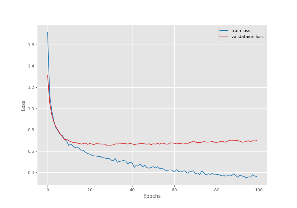
Following are the graphs for Mean IoU, pixel accuracy, and the loss during training & validation.
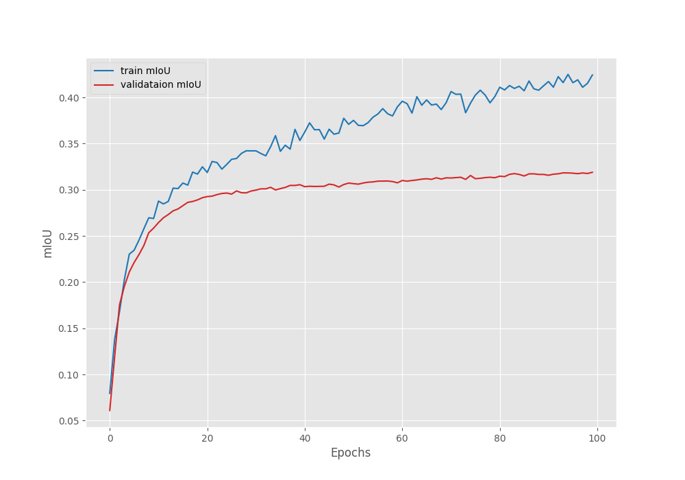
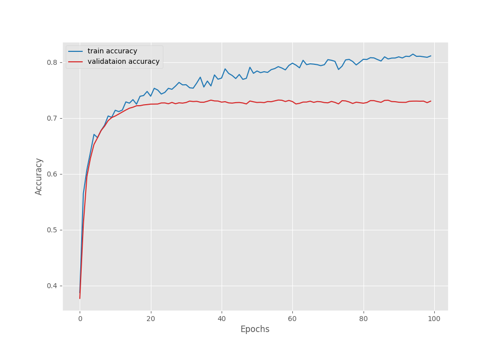
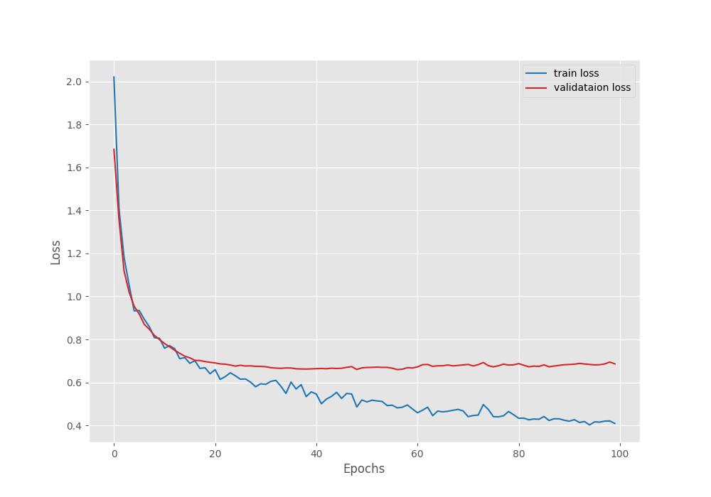
From the loss graph, it seems that the model started to overfit after 60 epochs. However, the validation plots of the accuracy and Mean IoU seem to be improving till the end of training.
Preparing Dataset by Splitting the Original Images
For the next experiment, we will generate a different version of the dataset. We do not have too many samples in the dataset, just 120 for training. However, the original images are 1241 pixels wide and 370 pixels in height. We can divide each image and generate two images, one covering the right side of the scene, and the other covering the left side of the scene.
We can achieve this through the create_data_folder_half_image.py script. Here are its contents.
import os
import shutil
import cv2

from tqdm.auto import tqdm

splits = ['train', 'val']
DST_DIR = '../input/split_data_half'
IMG_DIR = os.path.join(DST_DIR, 'images')
LBL_DIR = os.path.join(DST_DIR, 'labels')

ROOT_IMG_DIR = '../input/images'
ROOT_LBL_DIR = '../input/labels'

os.makedirs(DST_DIR, exist_ok=True)
for split in splits:
    os.makedirs(os.path.join(IMG_DIR, split), exist_ok=True)
for split in splits:
    os.makedirs(os.path.join(LBL_DIR, split), exist_ok=True)

train_file = open('../input/splits/train.txt', 'r')
train_images = train_file.readlines()
train_images = [train_image.rstrip().split('images/')[-1] for train_image in train_images]
print(train_images)

test_file = open('../input/splits/test.txt', 'r')
test_images = test_file.readlines()
test_images = [test_image.rstrip().split('images/')[-1] for test_image in test_images]
print(test_images)

# Copy data to respective directories.
def copy(split='train', data_list=None):
    for data in tqdm(data_list, total=len(data_list)):
        data_name = data.split('.pcd')[0]
        image_path = os.path.join(ROOT_IMG_DIR, data_name+'.png')
        label_path = os.path.join(ROOT_LBL_DIR, data_name+'.png')

        image = cv2.imread(image_path)
        label = cv2.imread(label_path)

        if split == 'train':
            # As each image is 1241 pixels in widht, this will generate images
            # and labels of 827 in width and 370 in height. Each image and
            # label will have a slight overlap ensuring that the entire road
            # is covered in each half of the image.
            image_left = image[0:image.shape[0], 0:int(image.shape[1]//1.5)]
            image_right = image[0:image.shape[0], image.shape[1]-int(image.shape[1]//1.5):image.shape[1]]

            label_left = label[0:label.shape[0], 0:int(label.shape[1]//1.5)]
            label_right = label[0:label.shape[0], label.shape[1]-int(label.shape[1]//1.5):label.shape[1]]

            cv2.imwrite(
                os.path.join(IMG_DIR, split, data_name+'_left.png'), image_left
            )
            cv2.imwrite(
                os.path.join(IMG_DIR, split, data_name+'_right.png'), image_right
            )

            cv2.imwrite(
                os.path.join(LBL_DIR, split, data_name+'_left.png'), label_left
            )
            cv2.imwrite(
                os.path.join(LBL_DIR, split, data_name+'_right.png'), label_right
            )

        else:
            shutil.copy(
            image_path,
            os.path.join(IMG_DIR, split, data_name+'.png')
            )
            shutil.copy(
                label_path,
                os.path.join(LBL_DIR, split, data_name+'.png')
            )

copy(split='train', data_list=train_images)
copy(split='val', data_list=test_images)
In the above script, the logic behind dividing each image into two scenes is present from lines 41 to 64.
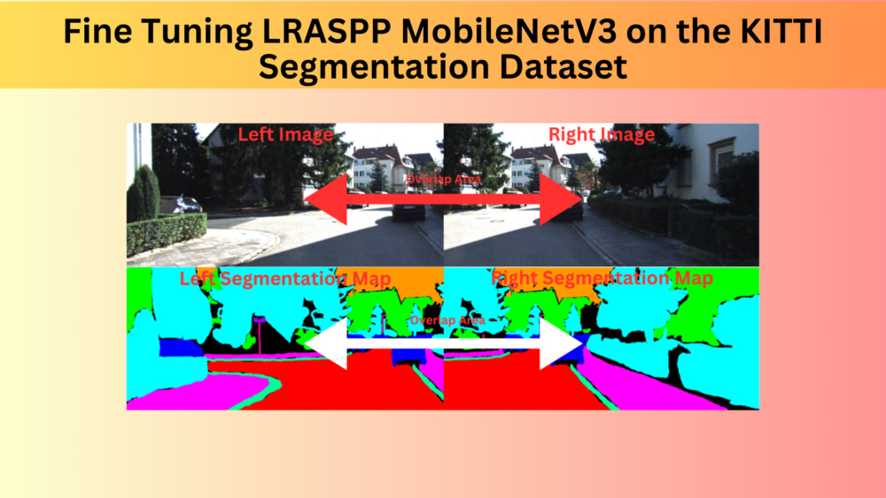
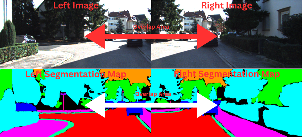
We simply divide each image into two parts of 370×827 resolution. After this, we have a left image and a right image from each original image. Notice that the left and right scenes after this have an overlap because we are not dividing the image in the middle. This is to ensure that each side of the image contains the entire road. This is necessary as the model needs to see the entire road to learn to segment it properly. In spite of this overlap, there is enough variability in each image.
We can execute the script to generate the split images dataset.
python create_data_folder_half_image.py
Here is a sample, showing the left and right sides of an image along with the approximate overlap area.
This provides us with a larger dataset for training, 240 training samples to be particular. However, we do not modify the validation samples. This is to ensure that we can compare the metrics with the ones from the original training earlier.
Fine Tuning the LRASPP MobileNetV3 Segmentation Model on the Divided Images
Now, let’s run the training experiment on the new set of data.
python train.py --batch 8 --height 376 --width 1240 --lr 0.05 --epochs 100 --out split_training --data ../input/split_data_half/
All the command line arguments remain the same, except the path to the training data folder which now points to the new directory.
This time, the model reached the best Mean IoU of 33.65% on epoch 99.
EPOCH: 99
Training
100%|████████████████████| 30/30 [00:06<00:00,  4.34it/s]
Validating
100%|████████████████████| 11/11 [00:02<00:00,  4.36it/s]

Best validation IoU: 0.3365676607465478

Saving best model for epoch: 99

Train Epoch Loss: 0.3662, Train Epoch PixAcc: 0.8505, Train Epoch mIOU: 0.441163
Valid Epoch Loss: 0.6954, Valid Epoch PixAcc: 0.7372 Valid Epoch mIOU: 0.336568
We have an increment of 1.75% compared to the previous training. Here are the Mean IoU, accuracy, and loss graphs from the above training experiments.
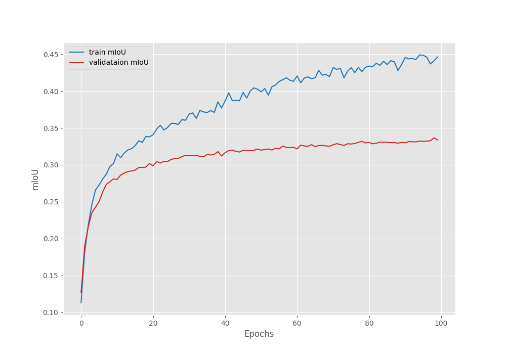
This time also, the accuracy and Mean IoU graphs seem to be improving till the end of training whereas the validation loss points towards overfitting of the model. Still, we will use the model saved according to the best Mean IoU for inference.
This concludes all the fine tuning experiments for the LRASPP model. Next, we will move on to running inference on some real-world driving footage.
Inference using the Best LRASPP MobileNetV3 Model Fine Tuned on the Original Images
Let’s run inference using the best validation IoU-weights that we obtained by training the LRASPP MobileNetV3 on the original images.
We will run inference on videos using the inference_video.py script.
The inference videos are present in the input/inference_data directory.
python inference_video.py --input ../input/inference_data/video_1.mov --out ../outputs/inference_normal_training --model ../outputs/normal_training/best_model_iou.pth
Following are the results.
The RTX 3080 GPU can run the model at 43 FPS on average. Now, coming to the qualitative analysis of the results.
It is obvious that we are not getting fine-grained segmentation using the model. The model is able to segment the road and cars, with patches of other segmentation objects though. It is also able to segment trees and buildings but with a lot of flickering.
Inference using the Best LRASPP MobileNetV3 Model Fine Tuned on the Split Images
Let’s now use the best model from the second run where we trained the model using split-images. First, we will run inference using the same video as above to draw a comparison.
python inference_video.py --input ../input/inference_data/video_1.mov --out ../outputs/inference_split_training --model ../outputs/split_training/best_model_iou.pth
From an initial look, the results look the same. However, we can draw a side-by-side comparison to get better insights.
Side-by-Side Comparison of Trained LRASPP Models for Video Segmentation Results
Here is a side-by-side comparison of both the inference runs.
Two things become apparent from the above video clip. The model trained with the split-images segments the cars and buildings slightly better than the other model. We can attribute this to the mode data that it got to see during training. Despite that, both models are making mistakes while segmenting the road and sidewalks. So, neither of them are overly good at the moment.
Let’s check another comparison.
In this case, also, the model trained with split-images is segmenting the cars and the road much better. However, just like the previous comparison, neither of them is perfect.
From the above training and inference experiments, we can conclude one thing. The quantity and quality of training data both matter in training a good segmentation model. Even if we use a smaller model like LRASPP MobileNetV3, we can obtain much better results with more high-quality training data. In the next article, we will train the model on a larger Autonomous Driving Scene Segmentation dataset and try to obtain even better results.
Summary and Conclusion
In this article, we fine tuned the LRASPP MobileNetV3 segmentation model on the KITTI dataset. While training, we observed some inherent issues with smaller datasets and tried to mitigate that to some extent as well. In the next article, we will cover training better models and continue on the topic. I hope that this article was worth your time.
If you have any doubts, thoughts, or suggestions, please leave them in the comment section. I will surely address them.
You can contact me using the Contact section. You can also find me on LinkedIn, and X.

3 thoughts on “Fine Tuning LRASPP MobileNetV3 on the KITTI Segmentation Dataset”