Qwen2 VL – Inference and Fine-Tuning for Understanding Charts

Vision-Language understanding models are playing a crucial role in deep learning now. They can help us summarize, answer questions, and even generate reports faster for complex images. One such family of models is the Qwen2 VL. They have instruct models in the range of 2B, 7B, and 72B parameters. The smaller 2B models, although fast and require less memory, do not perform well on chart understanding. In this article, we will cover two aspects while dealing with the Qwen2 VL models – inference and fine-tuning for understanding charts.

We will use the Unsloth library to create the inference and fine-tuning pipelines. After training the model, we will create a Gradio application to chat with the model easily.

What will we cover with Qwen2 VL?

• We will start with a brief background of the Qwen2 VL from the official report.
• Next, we will move to understanding the dataset we will use for fine-tuning.
• Before moving to the training phase, we will analyze the performance of the pretrained model using a few images from the validation dataset. This will give us an idea of where the model is failing.
• Next, we will move to fine-tuning:
  • We will start with loading the model and preparing the dataset.
  • We will also cover some caveats of the image preparation code and how to manage RAM and VRAM, particularly OOM issues.
• After training, we will create a Gradio application to chat with the model.

The Qwen2 VL Model

The Qwen2 VL model is the result of the continued development of the Qwen2 LLM.

The model uses the same language decoder as Qwen2. For the vision encoder, it employs a pretrained ViT from DFN (Data Filtering Networks).

The Qwen2 VL has three different parameter sizes, 2B, 7B, and 72B.

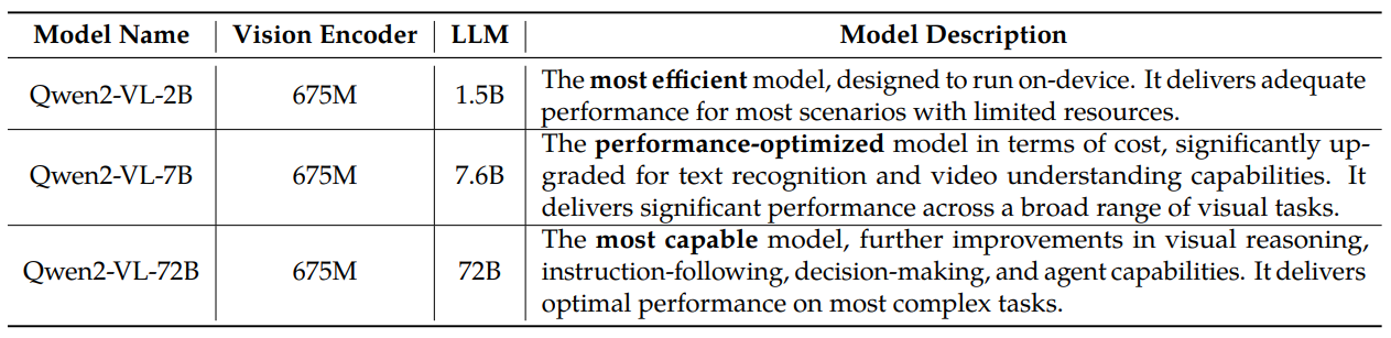
However, the size of the vision encoder remains the same (675M parameters) across all models. This ensures a consistent computational load across all sizes. This is in contrast to the Llama 3 vision model where the image encoder and cross-attention modules account for ~25% increase in parameters depending on the size of the language decoder.

Let’s discuss some of the architectural innovations of the Qwen2 VL model.

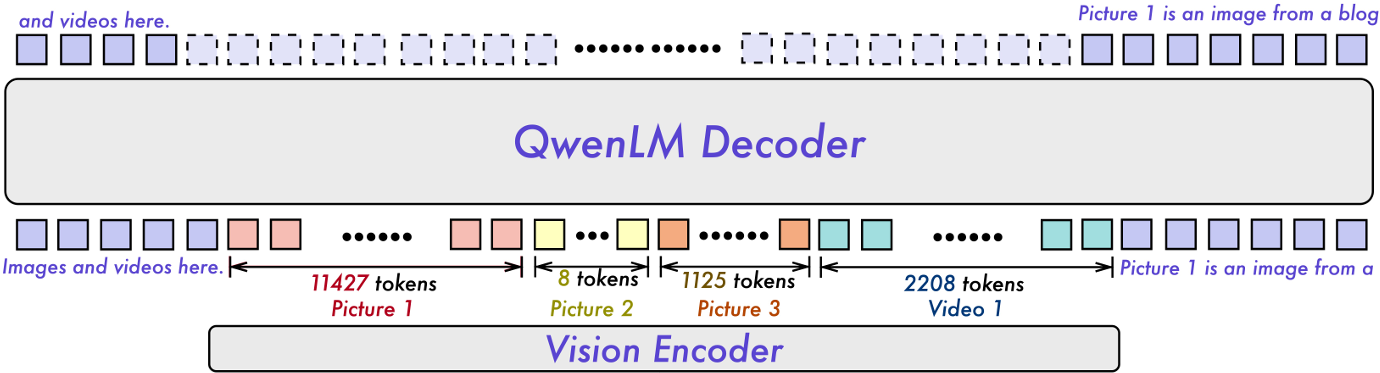
Naive Dynamic Resolution

The naive dynamic resolution in Qwen2 VL is a step up from its predecessor, Qwen VL. This feature allows the model to process images of any resolution and convert them into a dynamic number of visual tokens.

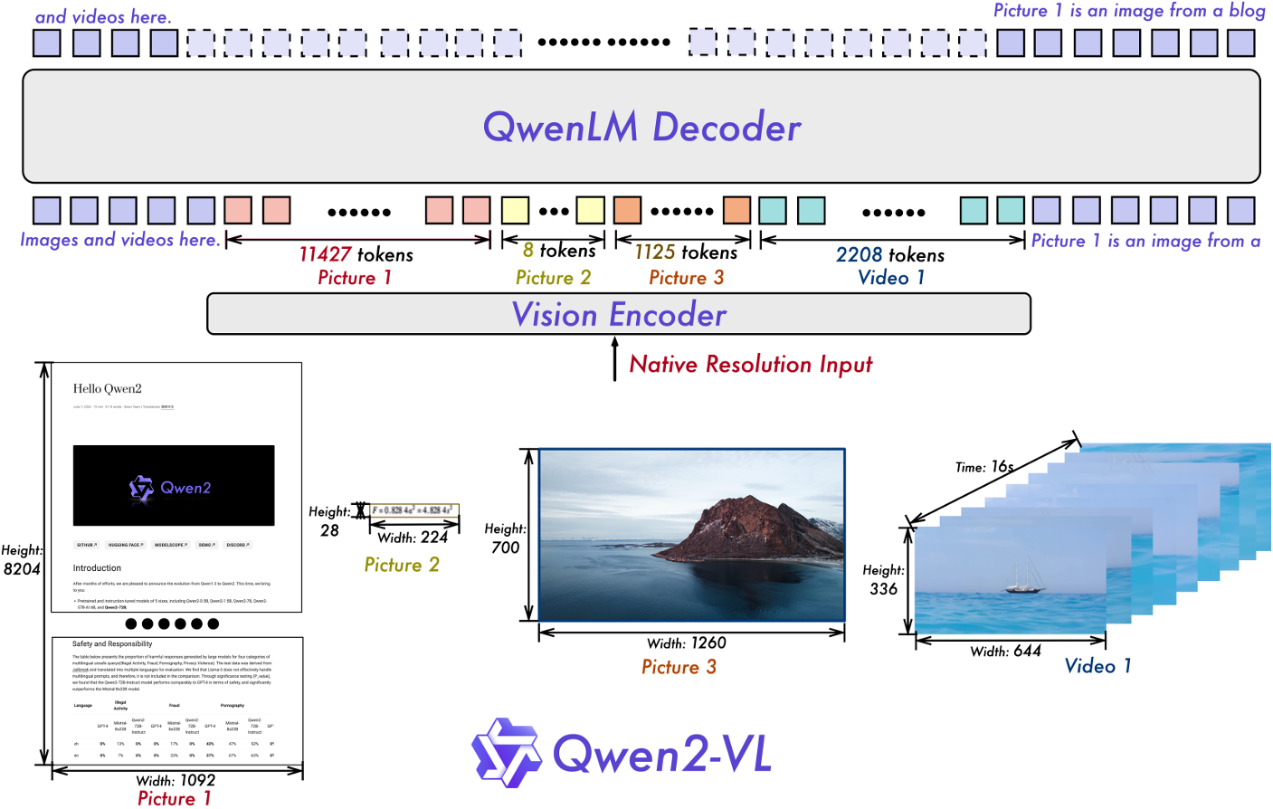
This requires a modification to the original Vision Transformer architecture. Instead of using absolute positional encodings, the authors employ a new 2D-RoPE (2D-Rotary Positional Encoding) technique. This helps capture the 2D positional information of the images.

Multimodal Rotary Position Embedding (M-RoPE)

The M-RoPE is another key architectural change for the language decoder.

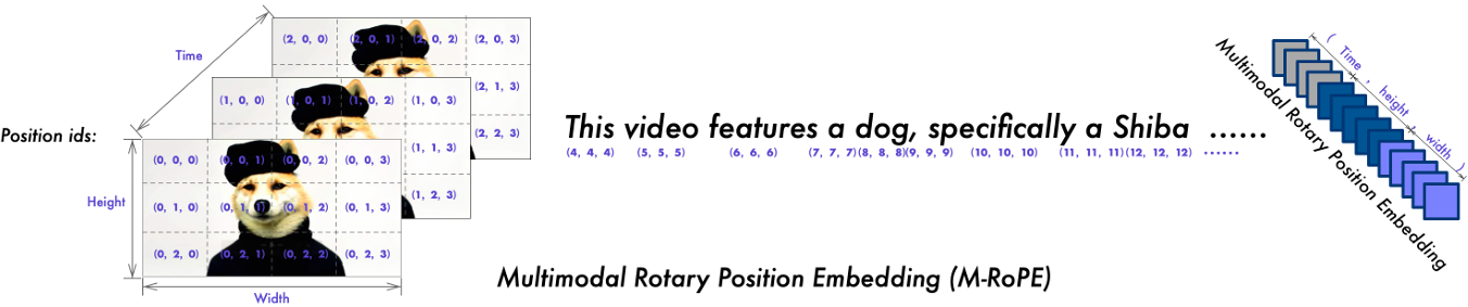
Traditionally, LLMs use 1D-RoPE. This limits the positional information to one dimension. However, with M-RoPE, the Qwen2 VL model can include positional information of multimodal inputs. For this, the input is deconstructed into three components: temporal (time), height, and width.

For text input, M-RoPE acts identically to 1D-RoPE. However, when processing images, it helps encode the distinct IDs for the height and width while keeping the temporal IDs constant. When processing videos, the temporal ID of each frame is incremented.

Unified Image and Video Understanding

During training, Qwen2 VL uses both image and video data instead of training separately. Furthermore, the authors use 3D convolutions to process video data which helps to process more video frames without increasing the sequence length.

Interesting Findings and Caveats

Here are some interesting findings and caveats that I found out while experimenting with Qwen2 VL.

Qwen2 VL is great at formula parsing. Although this was the initial course of fine-tuning, after testing even the 2B model, I did not feel a need to train it further. Of course, the authors also mention that it has been trained on math, code, and equation data and is quite good at parsing mathematical equations.

However, it falls short of chart understanding and connecting the text in the charts’ legends or axes to the visual content. This is why we will fine-tune the Qwen2 VL 2B model further for better chart understanding.

Above, we discussed that Qwen2 VL uses a naive dynamic resolution scaling for images, which, although good for extracting important information, can cause huge memory spikes. Further in the article, we will see how to mitigate this issue while inferencing and fine-tuning.

The Pixmo Docs (Charts) Dataset

We will be fine-tuning the Qwen VL model on the Pixmo Docs dataset released by AllenAI (Ai2). This is part of the dataset that the Molmo VLM was trained on.

We will train the Qwen2 VL on the Charts subset of the dataset. You can find the dataset here on HuggingFace.

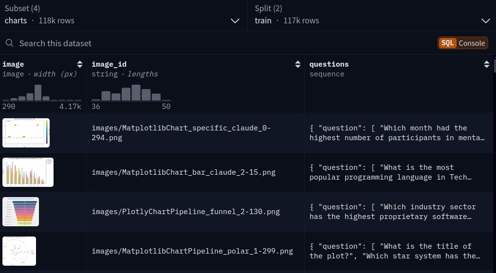
The dataset contains three columns: image, image_id, and questions.

Each question is a dictionary containing a question and an answer key. Following is a sample showing the image and the question as well.

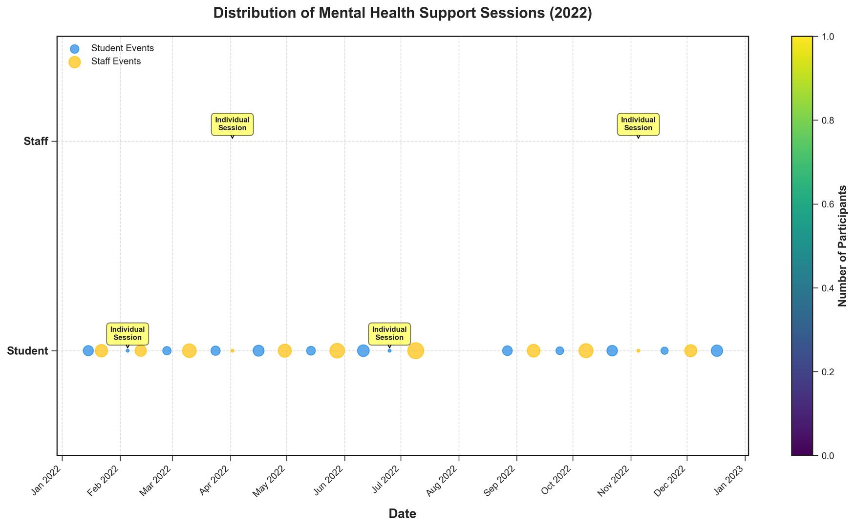
{ "question": [ "Which month had the highest number of participants in mental 
health support sessions?", "What is the total number of participants in staff 
events over the year?", "Compare the number of participants in individual 
counseling sessions for students versus staff. Which is higher?", "What is the 
average number of participants per event for student events?", "Which event 
had the maximum number of participants and how many?", "Are there more student 
events or staff/teacher events over the year?", "Do student events tend to have 
participants more or less than staff events?", "What month had the highest 
diversity of event types (student and staff events)?", "Which quarter of the 
year saw the highest number of student events?" ], "answer": [ "August", "219", 
"Equal", "Approximately 9.46", "Summer Staff Wellness Retreat, 30", "Student 
Events", "Less", "April", "Q4" ] }

Each of the keys contains a list of questions and corresponding answers respectively.

There are around 117,000 training samples and around 1,020 validation samples. We will use a subset of the dataset for training.

Project Directory Structure

Let’s take a look at the project directory structure.

├── input
│   ├── image_1.jpg
│   ├── image_2.jpg
│   └── image_3.jpg
├── outputs
│   ├── checkpoint-2000
│   └── checkpoint-2500
├── app.py
├── qwen_2_vl_2b_fine_tuning.ipynb
└── qwen_2_vl_2b_pretrained_inference.ipynb

• The input directory contains the images that we will use for inference and testing after fine-tuning the model.
• The outputs directory contains the checkpoints from fine-tuning.
• We have two notebooks: one inference notebook that uses the pretrained model and one fine-tuning notebook. The app.py script contains the code for the Gradio application.

The article provides a downloadable zip file containing all the code files, the pretrained models, a README file containing the installation steps, and the inference images.

Download Code

Installing Dependencies

Let’s install all the requirements needed for fine-tuning Qwen2 VL.

• Create an Anaconda Environment and install PyTorch and xformers with CUDA support.

conda create --name unsloth_env \
    python=3.11 \
    pytorch-cuda=12.1 \
    pytorch cudatoolkit xformers -c pytorch -c nvidia -c xformers \
    -y

conda activate unsloth_env

• Next, we will install a slightly older version of Unsloth. As of writing this, the latest version of Unsloth had embedding layers error when initializing the Qwen2 VL model.

pip install --no-cache-dir unsloth==2024.12.11
pip install --no-cache-dir unsloth_zoo==2024.12.6

• Install the rest of the Hugging Face dependencies.

pip install --no-deps trl peft accelerate bitsandbytes

The zip file that comes with the post also contains a README.md file laying out the steps to install the requirements.

Inference Using the Qwen2 VL 2B Pretrained Model

We will start with inference experiments using the pretrained model. We will use the 2B model in 4-bit quantized format.

All the code discussed in this section is present in the qwen_2_vl_2b_pretrained_inference.ipynb Jupyter Notebook.

Unsloth streamlines VLM inference and fine-tuning. Therefore, a lot of code will remain similar to what we discussed in the Llama 3.2 Vision inference and Llama 3.2 Vision fine-tuning articles. I highly recommend going through the code explanation in the above mentioned articles. Here, we will discuss the important parts of the code only.

The inference shown here was run on a system with 10GB RTX 3080 GPU, 32GB RAM, and i7 10th generation processor.

Import Statements

Let’s import all the necessary libraries and modules.

from unsloth import FastVisionModel
from transformers import TextStreamer
from PIL import Image

import torch

Load the Model for Inference and Initialize the Text Streamer

We will use the FastVisionModel class to load the model in quantized format and text streamer for streaming output.

model, tokenizer = FastVisionModel.from_pretrained(
    'unsloth/Qwen2-VL-2B-Instruct',
    load_in_4bit=True
)

text_streamer = TextStreamer(tokenizer, skip_prompt=True, skip_special_tokens=True)

FastVisionModel.for_inference(model)

Helper Function for Inference

The following describe_image function loads an image, prepares the instruction, and passes it through the Qwen2 VL model.

def describe_image(image_path, instruction='Describe the image accurately.'):
    messages = [
        {'role': 'user', 'content': [
            {'type': 'image'},
            {'type': 'text', 'text': instruction}
        ]}
    ]
    
    image = Image.open(image_path)
    image = image.resize((1024, 768))

    input_text = tokenizer.apply_chat_template(messages, add_generation_prompt=True)
    inputs = tokenizer(
        image,
        input_text,
        add_special_tokens=False,
        return_tensors='pt',
    ).to('cuda')

    _ = model.generate(
        **inputs, 
        streamer=text_streamer, 
        max_new_tokens=1024,
        use_cache=True, 
        temperature=1.5, 
        min_p=0.1
    )

Notice that we are resizing the model to 768×1024 (height x width) resolution. This is to mitigate the memory spike issue that we discussed earlier. The memory spike happens due to the naive dynamic resizing employed by the Qwen2 VL’s image processor. So, resizing it manually ensures constant VRAM usage. This leads the code to run on even 8GB of VRAM with excellent results.

Call the Function to Run Inference

We can call the function with an image path and an instruction to run inference. Following is an example.

describe_image(
    'input/image_1.jpg', 
    instruction='What does the image show?'
)

Discussion of Pretrained Model’s Inference Results

Before moving to the fine-tuning section, let’s discuss a few results from the pretrained model. This will show the model’s strengths and weaknesses for better analysis. We are using images from the validation set of the Pixmo Charts dataset.

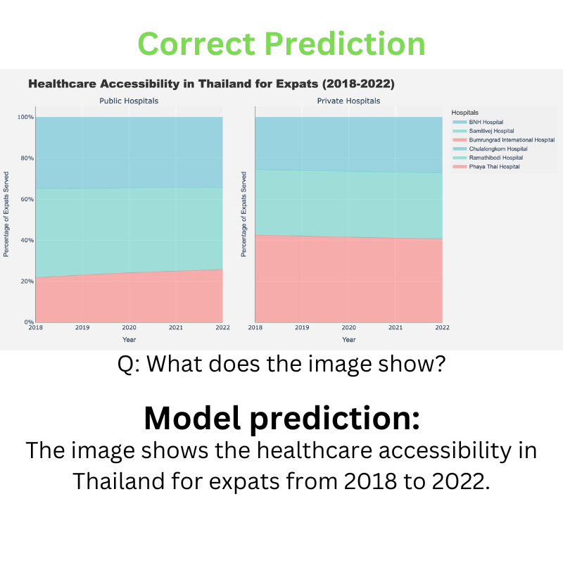
The above figure shows a correct prediction where we ask the model to describe the image. It was a straightforward question for an initial assessment.

Let’s try a difficult question now.

In this case, the model had to analyze the chart properly, match the legend on the right with the area of the graph, and answer the question. This is a much more difficult use case and the model failed here. The correct answer is Bumrungrad International Hospital.

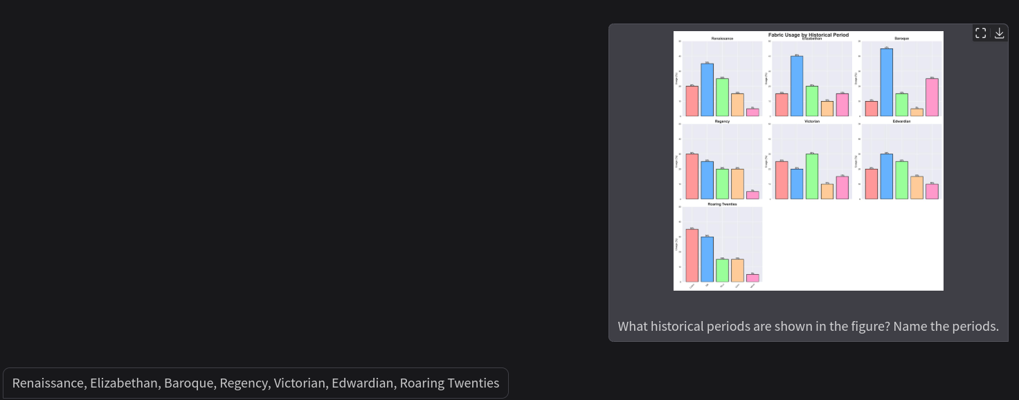
A final question where the model has to analyze bar charts.

The model answers the question incorrectly here as the Elizabethan period whereas the correct answer is the Baroque period.

In fact, when the model was prompted to mention all the historical periods mentioned in the chart, it mentioned the Roaring Twenties twice. This indicates a failure in the spatial analysis of charts. Surely, fine-tuning the model will mitigate at least some of the issues and give us better results.

Fine-Tuning Qwen2 VL for Understanding Charts

The above results bring us to the fine-tuning section. We will use QLoRA technique for fine-tuning which uses minimal resources for a 2B parameter model.

The code for fine-tuning is present in the qwen_2_vl_2b_fine_tuning.ipynb Jupyter Notebook.

Most of the code remains similar to the Llama 3.2 Vision fine-tuning. We will only discuss the major changes here for the sake of brevity.

The fine-tuning shown here was run on an NVIDIA L4 GPU with 24 GB VRAM and it took approximately 5.5 hours for the training to complete.

Imports, Loading the Model, and Preparing it for Fine-Tuning

The following code block contains all the necessary imports, loading of the Qwen2 VL model, and preparing it for parameter efficient fine-tuning.

from unsloth import FastVisionModel
from tqdm import tqdm
from transformers import TextStreamer
from unsloth import is_bf16_supported
from unsloth.trainer import UnslothVisionDataCollator
from trl import SFTTrainer, SFTConfig
from datasets import load_dataset

import matplotlib.pyplot as plt
import torch

model, tokenizer = FastVisionModel.from_pretrained(
    'unsloth/Qwen2-VL-2B-Instruct',
    load_in_4bit=True,
    use_gradient_checkpointing='unsloth', # True or "unsloth" for long context
)

model = FastVisionModel.get_peft_model(
    model,
    finetune_vision_layers=True, # False if not finetuning vision layers
    finetune_language_layers=True, # False if not finetuning language layers
    finetune_attention_modules=True, # False if not finetuning attention layers
    finetune_mlp_modules=True, # False if not finetuning MLP layers

    r=16,           # The larger, the higher the accuracy, but might overfit
    lora_alpha=16,  # Recommended alpha == r at least
    lora_dropout=0,
    bias='none',
    random_state=3407,
    use_rslora=False,  # We support rank stabilized LoRA
    loftq_config=None, # And LoftQ
    # target_modules="all-linear", # Optional now! Can specify a list if needed
)

Loading the Pixmo Charts Dataset

Next, we need to load the Pixmo Charts dataset from Hugging Face.

dataset_train = load_dataset('allenai/pixmo-docs', 'charts', split='train[:20000]')
dataset_test = load_dataset('allenai/pixmo-docs', 'charts', split='validation[:1000]')

We are using 20000 samples for training and 1000 samples for validation.

Creating Instruction Prompt Template

We know that each image sample contains multiple questions and answers. So, we need a proper way to create question-and-answer pairs for each image. The following convert_to_conversation function does that.

instruction = 'Answer concisely based on the image and questions.'

def convert_to_conversation(sample):
    qna = ''

    for i in range(len(sample['questions']['question'])):
        qna += f'Q: {sample["questions"]["question"][i]}\nA: {sample["questions"]["answer"][i]}\n'
    
    image = sample['image'].resize((416, 416))

    conversation = [
        { 'role': 'user',
          'content' : [
            {'type' : 'text',  'text'  : instruction},
            # {'type' : 'image', 'image' : sample['image']} ]
            {'type' : 'image', 'image' : image} ]
        },
        { 'role' : 'assistant',
          'content' : [
            {'type' : 'text',  'text'  : qna} ]
        },
    ]
    return { 'messages' : conversation }

For each sample, we loop through the number of questions. Each question is prepended with Q: and after a new line each answer is prepended with A:. All such question-answer pairs are present in a new line.

Furthermore, notice that we are resizing the images to 416×416 resolution for fine-tuning. This is in contrast to the Llama 3.2 Vision fine-tuning where we need not resize images. The image processor of Llama 3.2 Vision handled that efficiently. From experiments, I found that this serves a good balance between VRAM usage and accuracy. Higher resolution will lead to a spike in VRAM usage and any lower resolution than this will lead to a loss of details in the charts.

In fact, if you are training on a high VRAM machine (e.g. 48GB VRAM), try resizing the images to 1024×1024 and keeping the batch size as 8. That will give even better results.

Next, we need to map the sample to the above function.

converted_dataset_train = [
    convert_to_conversation(sample) \
    for sample in tqdm(dataset_train, total=len(dataset_train))
]

converted_dataset_test = [
    convert_to_conversation(sample)
    for sample in tqdm(dataset_test, total=len(dataset_test))
]

Printing a sample from the converted dataset gives the following result.

{'messages': [{'role': 'user', 'content': [{'type': 'text', 'text': 'Answer 
concisely based on the image and questions.'}, {'type': 'image', 'image': 
<PIL.Image.Image image mode=RGB size=416x416 at 0x7FE2CDBC6080>}]}, {'role': 
'assistant', 'content': [{'type': 'text', 'text': 'Q: Which month had the 
highest number of participants in mental health support sessions?\nA: 
August\nQ: What is the total number of participants in staff events over the 
year?\nA: 219\nQ: Compare the number of participants in individual counseling 
sessions for students versus staff. Which is higher?\nA: Equal\nQ: What is 
the average number of participants per event for student events?\nA: 
Approximately 9.46\nQ: Which event had the maximum number of participants and 
how many?\nA: Summer Staff Wellness Retreat, 30\nQ: Are there more student 
events or staff/teacher events over the year?\nA: Student Events\nQ: Do student 
events tend to have participants more or less than staff events?\nA: Less\nQ: 
What month had the highest diversity of event types (student and staff 
events)?\nA: April\nQ: Which quarter of the year saw the highest number of 
student events?\nA: Q4\n'}]}]}

As we can see, each question-answer pair is present in a new line format.

Training the Qwen2 VL Model

For training, we need to enable the training mode in Unsloth and define all the trainer arguments.

FastVisionModel.for_training(model) # Enable for training!

trainer = SFTTrainer(
    model=model,
    tokenizer=tokenizer,
    data_collator=UnslothVisionDataCollator(model, tokenizer), # Must use!
    train_dataset=converted_dataset_train,
    eval_dataset=converted_dataset_test,
    args=SFTConfig(
        per_device_train_batch_size=8,
        per_device_eval_batch_size=8,
        gradient_accumulation_steps=1,
        warmup_steps=10,
        # max_steps=800,
        num_train_epochs=1, # For full training runs over the dataset.
        learning_rate=2e-4,
        fp16=not is_bf16_supported(),
        bf16=is_bf16_supported(),
        logging_steps=500,
        eval_strategy='steps',
        eval_steps=500,
        save_strategy='steps',
        save_steps=500,
        save_total_limit=2,
        optim='adamw_8bit',
        weight_decay=0.01,
        lr_scheduler_type='linear',
        seed=3407,
        output_dir='outputs',
        report_to='none',     # For Weights and Biases
        load_best_model_at_end=True,
        remove_unused_columns=False,
        dataset_text_field='',
        dataset_kwargs={'skip_prepare_dataset': True},
        dataset_num_proc=8,
        max_seq_length=2048,
        dataloader_num_workers=8
    ),
)

We will be training for a single epoch with a batch size of 8. This occupies around 13.5 GB of VRAM. You may reduce the batch size and adjust the gradient accumulation steps for training on a machine with less VRAM.

Finally, we start the training.

trainer_stats = trainer.train()

Following are the training logs.

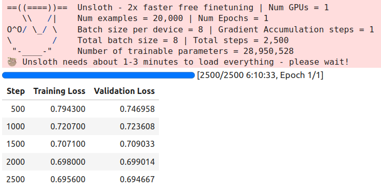
We will use the last saved checkpoint in the Gradio application for inference.

Inference Using the Gradio Application with the Fine-Tuned Qwen2 VL Model

The code for the Gradio application is present in app.py. However, we will not discuss the Gradio application code in detail here. This is primarily similar to the Llama 3.2 Vision Gradio application code with minimal changes.

One of the changes is loading the checkpoint of the pretrained model.

model, tokenizer = FastVisionModel.from_pretrained(
    model_name='outputs/checkpoint-2500',
    load_in_4bit=True
)

The second change is resizing the images in the describe_image function just as we did in the case of pretrained model inference.

def describe_image(user_input, history):
    print(user_input)
    messages = [
        {'role': 'user', 'content': [
            {'type': 'image'},
            {'type': 'text', 'text': user_input['text']}
        ]}
    ]
    
    input_text = tokenizer.apply_chat_template(messages, add_generation_prompt=True)

    image = Image.open(user_input['files'][0])
    image = image.resize((1024, 768))
.
.
.

Running the Script and Analyzing the Results

We can run the application by executing the script using the following command.

python app.py

Let’s discuss some of the results and check whether fine-tuning helped solve the issues that we had using the pretrained model.

We will start with the question about the healthcare accessibility chart and ask the same question about the hospital where the pretrained model responded incorrectly.

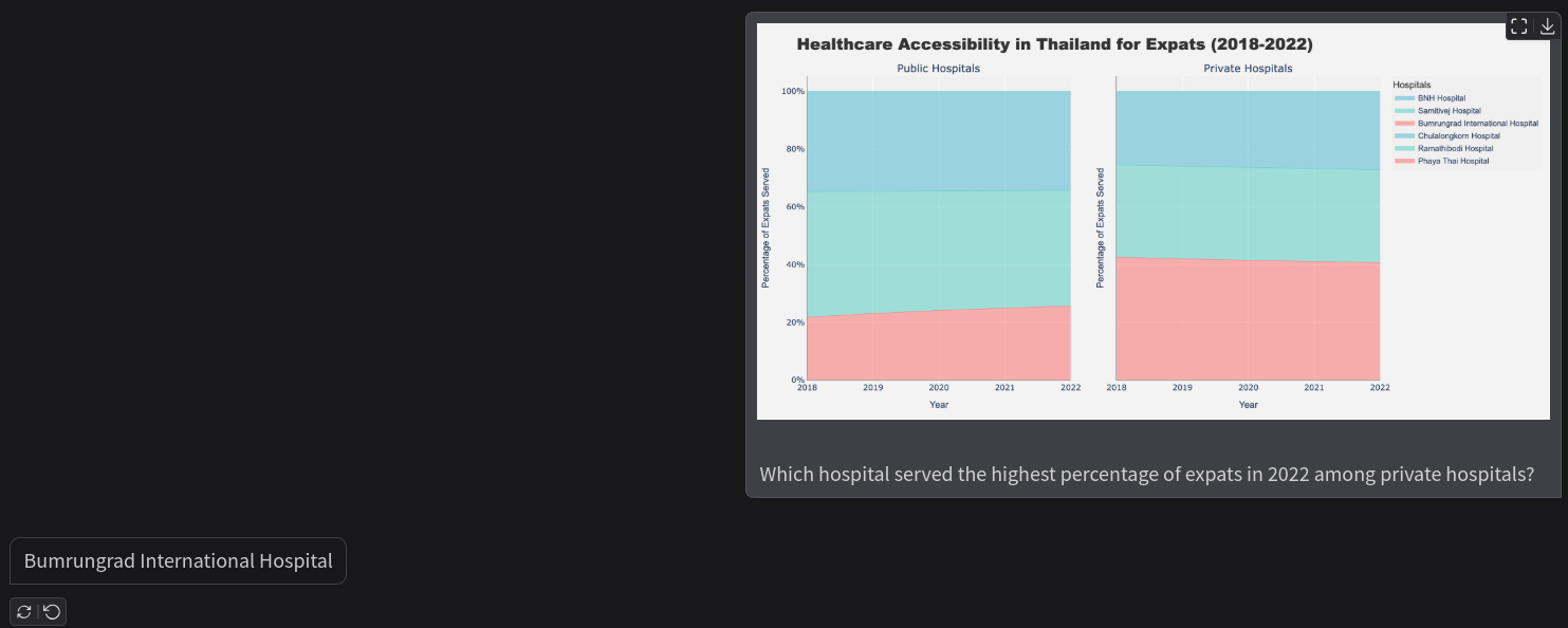
The model is answering the question correctly after fine-tuning. Note that these images are from the validation dataset, so, it seems that the model learned how to analyze and understand charts.

Next, we have two questions regarding the bar chart and fabric usage.

Previously, the model gave a partially correct answer to this question. However, now it is entirely correct showing that the spatial understanding has improved.

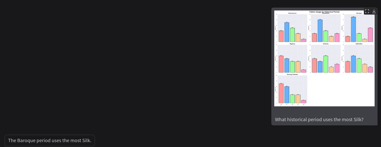
This time the answer is correct as well indicating that the model learned how to analyze the size of the bar plots.

Summary and Conclusion

In this article, we discussed the Qwen2 VL model. Starting with a brief understanding of the architecture, we also covered inference and fine-tuning for chart understanding. We experienced firsthand how training the model on chart images improved its spatial analysis of plots, legends, and axes. Of course, a more robust evaluation maybe needed for properly understanding the implications, however, this is a good starting point. I hope this article was worth your time.

If you have any questions, thoughts, or suggestions, please leave them in the comment section. I will surely address them.

You can contact me using the Contact section. You can also find me on LinkedIn, and Twitter.

References

• Qwen2-VL: Enhancing Vision-Language Model’s Perception of the World at Any Resolution
• Data Filtering Networks