

Although DINOv2 offers powerful pretrained backbones, training it to be good at semantic segmentation tasks can be tricky. Just training a segmentation head may give suboptimal results at times. In this article, we will focus on two points: multi-class semantic segmentation using DINOv2 and comparing the results with just training the segmentation and fine-tuning the entire network.
In previous articles about DINOv2, we have covered two aspects:
- Image classification using DINOv2 where we compare the results between fine-tuning and transfer learning.
- Training a segmentation head on top of DINOv2 features for person segmentation.
In this article, we will take it a step further and fine-tune the model on a multi-class segmentation dataset. Along the way, we will carry out two experiments and compare the results.
What will we cover while training DINOv2 for multi-class segmentation?
- We will start with the dataset discussion. We will use the Pascal VOC segmentation dataset here.
- Next, we will set up the training code. We will compare the modified code parts to the previous segmentation article on DINOv2.
- We will run two experiments:
- Training the segmentation head only.
- Fine-tuning the entire network.
- Finally, we will analyze the results.
The Pascal VOC Semantic Segmentation Dataset
We will run our training experiments for the DINOv2 multi-class segmentation on the Pascal VOC segmentation dataset.
You can download the dataset from here on Kaggle.
Following is the dataset directory structure, after downloading and extracting the dataset.
voc_2012_segmentation_data/
├── train_images  [1464 entries exceeds filelimit, not opening dir]
├── train_labels  [1464 entries exceeds filelimit, not opening dir]
├── valid_images  [1449 entries exceeds filelimit, not opening dir]
└── valid_labels  [1449 entries exceeds filelimit, not opening dir]
The dataset contains 1464 training images & mask pairs and 1449 validation images & mask pairs.
Here are a few samples.
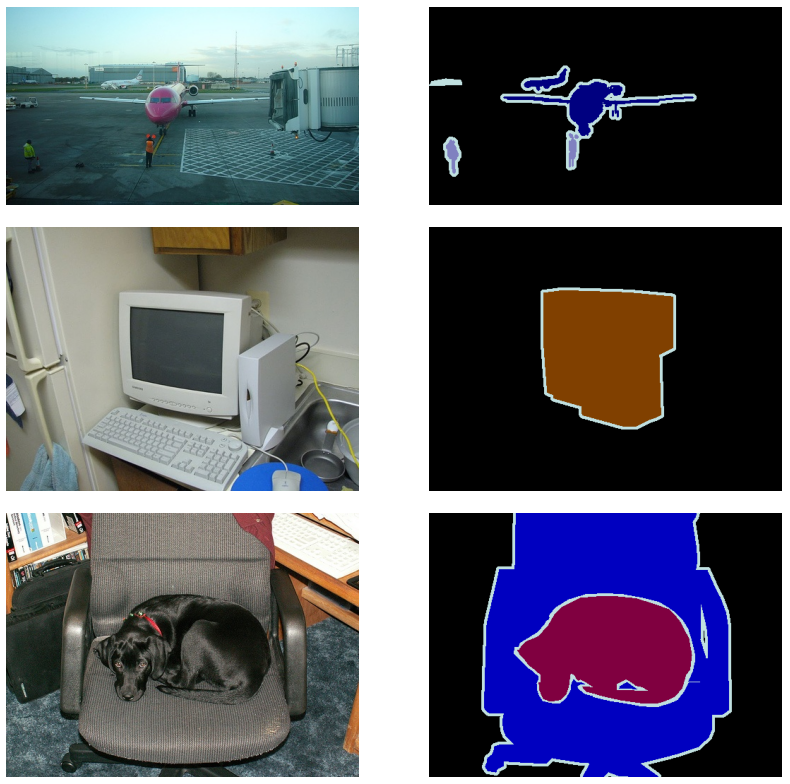
The dataset contains 21 classes including the background class.
[
    'background',
    'aeroplane',
    'bicycle',
    'bird',
    'boat',
    'bottle',
    'bus',
    'car',
    'cat',
    'chair',
    'cow',
    'dining table',
    'dog',
    'horse',
    'motorbike',
    'person',
    'potted plant',
    'sheep',
    'sofa',
    'train',
    'tv/monitor'
]
For each class, we have an RGB color segmentation mapping.
[
    [0, 0, 0],
    [128, 0, 0],
    [0, 128, 0],
    [128, 128, 0],
    [0, 0, 128],
    [128, 0, 128],
    [0, 128, 128],
    [128, 128, 128],
    [64, 0, 0],
    [192, 0, 0],
    [64, 128, 0],
    [192, 128, 0],
    [64, 0, 128],
    [192, 0, 128],
    [64, 128, 128],
    [192, 128, 128],
    [0, 64, 0],
    [128, 64, 0],
    [0, 192, 0],
    [128, 192, 0],
    [0, 64, 128]
]
Getting good results by directly training a segmentation model only using an ImageNet pretrained backbone on this dataset is difficult. This is because although the dataset contains variety the number of samples is less.
Furthermore, after carrying out the training experiments, we will analyze how training the segmentation head only and fine-tuning the entire DINOv2 segmentation network affect the results.
The Project Directory Structure
Let’s take a look at the project directory structure.
├── input
│   ├── inference_data
│   └── voc_2012_segmentation_data
├── notebooks
│   └── visualize.ipynb
├── outputs
│   ├── fine_tuning
│   ├── inference_results_video
│   └── transfer_learning
├── config.py
├── datasets.py
├── engine.py
├── infer_image.py
├── infer_video.py
├── metrics.py
├── model_config.py
├── model.py
├── requirements.txt
├── train.py
└── utils.py
- The
inputdirectory contains the training and inference data. - The
outputsdirectory contains the results after training the model and also the inference results. - In the project root directory, we have all the Python files that we need for training the DINOv2 segmentation model. Among these, we will focus on the
model.pyfile here.
The trained models, code files, and inference data are available via the download section. To train the model, please download the dataset from Kaggle and arrange it in the above directory structure.
Download Code
Installing Dependencies
After downloading the code file and extracting it, you can install the dependencies using the requirements file.
pip install -r requirements.txt
Now, let’s jump into the coding section of the article.
Multi-Class Semantic Segmentation using DINOv2
We will primarily discuss the model building code in this article. Most of the code is similar to what we discussed in one of our previous articles about DINOv2 semantic segmentation with transfer learning and fine-tuning experiments. This article simplified some of the model building components compared to the first DINOv2 segmentation article mentioned earlier.
Building the DINOv2 Semantic Segmentation Model
The code for model building resides in the model.py file.
Following are the imports that we need.
import torch
import torch.nn as nn

from functools import partial
from collections import OrderedDict
from torchinfo import summary
from model_config import model as model_dict
We import model configurations from the model_config module. This holds all the model configurations that were part of the original DINOv2 repository where the MMSegmentation library was used. Our approach simplifies the process and removes the MMSegmentation requirement entirely.
Next, we have a helper function to load the DINOv2 backbone.
def load_backbone(backbone_size="small"):
    backbone_archs = {
        "small": "vits14",
        "base": "vitb14",
        "large": "vitl14",
        "giant": "vitg14",
    }

    backbone_arch = backbone_archs[backbone_size]
    backbone_name = f"dinov2_{backbone_arch}"


    backbone_model = torch.hub.load(repo_or_dir="facebookresearch/dinov2", model=backbone_name)
    backbone_model.cuda()

    backbone_model.forward = partial(
        backbone_model.get_intermediate_layers,
        n=model_dict['backbone']['out_indices'],
        reshape=True,
    )

    return backbone_model
We use the DINOv2 Small backbone here for faster training. It contains around 22 million parameters.
We use a simple linear segmentation head where we reshape the output tokens to be fed into a final convolutional layer.
class LinearClassifierToken(torch.nn.Module):
    def __init__(self, in_channels, nc=1, tokenW=32, tokenH=32):
        super(LinearClassifierToken, self).__init__()
        self.in_channels = in_channels
        self.W = tokenW
        self.H = tokenH
        self.nc = nc
        self.conv = torch.nn.Conv2d(in_channels, nc, (1, 1))

    def forward(self,x):
        outputs =  self.conv(
            x.reshape(-1, self.in_channels, self.H, self.W)
        )
        return outputs
Then we have the final model building class that combines all the components.
class Dinov2Segmentation(nn.Module):
    def __init__(self, fine_tune=False):
        super(Dinov2Segmentation, self).__init__()

        self.backbone_model = load_backbone()
        print(fine_tune)
        if fine_tune:
            for name, param in self.backbone_model.named_parameters():
                param.requires_grad = True
        else:
            for name, param in self.backbone_model.named_parameters():
                param.requires_grad = False

        self.decode_head = LinearClassifierToken(in_channels=1536, nc=21, tokenW=46, tokenH=46)

        self.model = nn.Sequential(OrderedDict([
            ('backbone', self.backbone_model),
            ('decode_head', self.decode_head)
        ]))

    def forward(self, x):
        features = self.model.backbone(x)

        # `features` is a tuple.
        concatenated_features = torch.cat(features, 1)

        classifier_out = self.decode_head(concatenated_features)

        return classifier_out

if __name__ == '__main__':
    model = Dinov2Segmentation()

    summary(
        model,
        (1, 3, 644, 644),
        col_names=('input_size', 'output_size', 'num_params'),
        row_settings=['var_names']
    )
We have hard coded the number of classes to 21 here which matches the Pascal VOC dataset. However, it is much better to pass this as an argument while building the model.
We have discussed the nuances of building DINOv2 segmentation in our previous articles. Be sure to take a look at them if needed.
We can execute the file using the following command which will show us the network summary and parameters.
python model.py
=============================================================================================================================
Layer (type (var_name))                            Input Shape               Output Shape              Param #
=============================================================================================================================
Dinov2Segmentation (Dinov2Segmentation)            [1, 3, 644, 644]          [1, 21, 46, 46]           --
├─Sequential (model)                               --                        --                        --
│    └─DinoVisionTransformer (backbone)            [1, 3, 644, 644]          [1, 384, 46, 46]          526,848
│    │    └─PatchEmbed (patch_embed)               [1, 3, 644, 644]          [1, 2116, 384]            (226,176)
│    │    └─ModuleList (blocks)                    --                        --                        (21,302,784)
│    │    └─LayerNorm (norm)                       [1, 2117, 384]            [1, 2117, 384]            (768)
│    │    └─LayerNorm (norm)                       [1, 2117, 384]            [1, 2117, 384]            (recursive)
│    │    └─LayerNorm (norm)                       [1, 2117, 384]            [1, 2117, 384]            (recursive)
│    │    └─LayerNorm (norm)                       [1, 2117, 384]            [1, 2117, 384]            (recursive)
│    └─LinearClassifierToken (decode_head)         [1, 1536, 46, 46]         [1, 21, 46, 46]           --
│    │    └─Conv2d (conv)                          [1, 1536, 46, 46]         [1, 21, 46, 46]           32,277
=============================================================================================================================
Total params: 22,088,853
Trainable params: 32,277
Non-trainable params: 22,056,576
Total mult-adds (Units.MEGABYTES): 568.18
=============================================================================================================================
Input size (MB): 4.98
Forward/backward pass size (MB): 1047.40
Params size (MB): 86.25
Estimated Total Size (MB): 1138.63
=============================================================================================================================
The entire neural network contains around 22M parameters and the segmentation head contains 32,277 parameters.
Dataset Transforms and Training Hyperameters
We are using the following augmentations for the training dataset:
- Horizontal flipping
- Random brightness contrast
- Rotation
We will train the model using AdamW optimizer and use Cross Entropy as the loss function.
Transfer Learning Training using DINOv2 Semantic Segmentation Model
We will start with the transfer learning experiment.
python train.py --epochs 20 --imgsz 640 640 --out-dir transfer_learning --batch 2
We are training the model for 20 epochs with an image size of 640×640 and a batch size of 2. We choose a small batch size so that we can keep the same batch size for fine-tuning as well for comparable results.
Following are the results that we get.
EPOCH: 1
Training
100%|████████████████████| 366/366 [00:57<00:00,  6.36it/s]
Validating
100%|████████████████████| 363/363 [00:51<00:00,  7.08it/s]

Best validation loss: 0.44906933225958146

Saving best model for epoch: 1


Best validation IoU: 0.14743237744729587

Saving best model for epoch: 1

Train Epoch Loss: 1.0304, Train Epoch PixAcc: 0.7609, Train Epoch mIOU: 0.080638
Valid Epoch Loss: 0.4491, Valid Epoch PixAcc: 0.8659 Valid Epoch mIOU: 0.147432
LR for next epoch: [0.0001]
.
.
.
EPOCH: 19
Training
100%|████████████████████| 366/366 [00:57<00:00,  6.39it/s]
Validating
100%|████████████████████| 363/363 [00:49<00:00,  7.32it/s]

Best validation loss: 0.17451634874808558

Saving best model for epoch: 19


Best validation IoU: 0.2059438504460826

Saving best model for epoch: 19

Train Epoch Loss: 0.3764, Train Epoch PixAcc: 0.9045, Train Epoch mIOU: 0.173220
Valid Epoch Loss: 0.1745, Valid Epoch PixAcc: 0.9373 Valid Epoch mIOU: 0.205944
LR for next epoch: [0.0001]
--------------------------------------------------
EPOCH: 20
Training
100%|████████████████████| 366/366 [00:57<00:00,  6.40it/s]
Validating
100%|████████████████████| 363/363 [00:49<00:00,  7.31it/s]

Best validation loss: 0.17373583238500045

Saving best model for epoch: 20

Train Epoch Loss: 0.3740, Train Epoch PixAcc: 0.9047, Train Epoch mIOU: 0.172485
Valid Epoch Loss: 0.1737, Valid Epoch PixAcc: 0.9365 Valid Epoch mIOU: 0.203901
LR for next epoch: [0.0001]
--------------------------------------------------
TRAINING COMPLETE
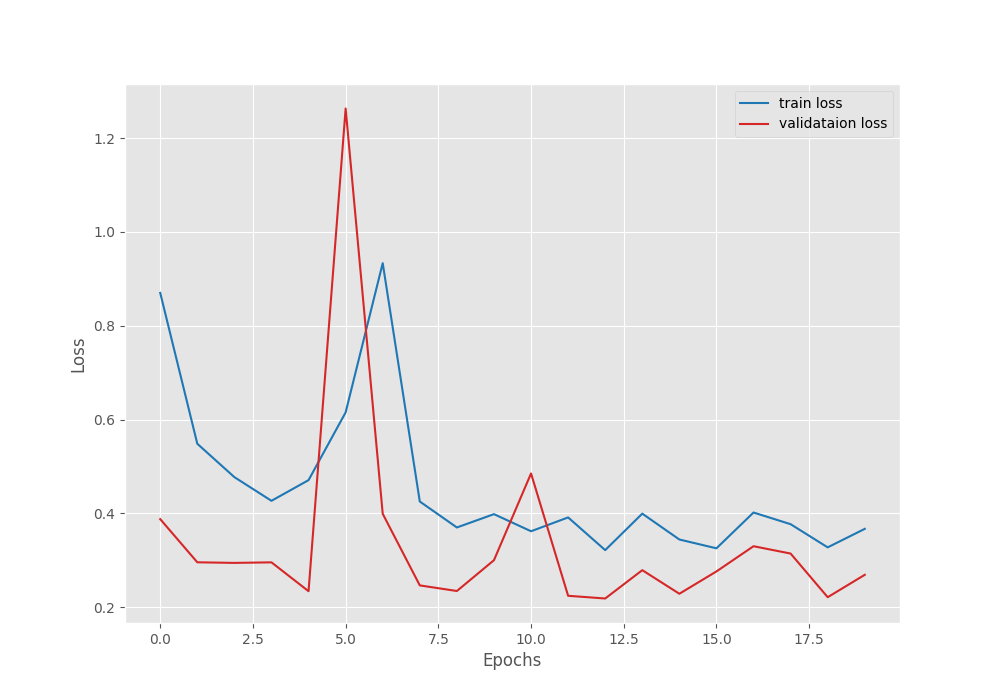
The model reaches the best validation mean IoU of 20.58%. Following are the loss, pixel accuracy, and mean IoU graphs.
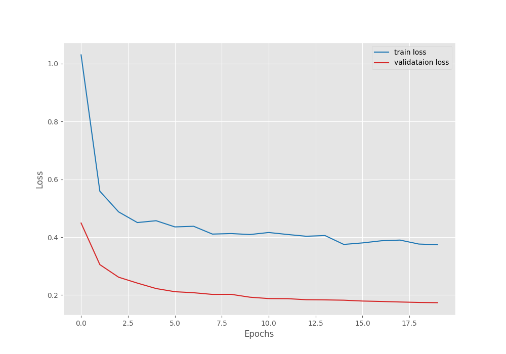
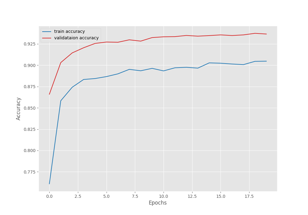
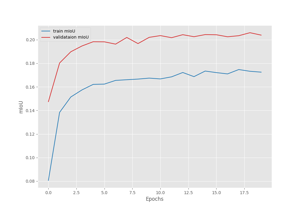
From the graphs, it is quite evident that the model has not converged yet and we can train it for longer.
Next, we will conduct the fine-tuning training experiment.
Fine-Tuning using DINOv2 Semantic Segmentation Model
To fine-tune the entire model, we just need to pass the --fine-tune command line argument additionally.
python train.py --epochs 20 --imgsz 640 640 --out-dir fine_tuning --fine-tune --batch 2 --lr 0.00001
However, this time, we start with a lower learning rate of 0.00001 to stabilize the training.
.
.
.
EPOCH: 19
Training
100%|████████████████████| 732/732 [02:20<00:00,  5.21it/s]
Validating
100%|████████████████████| 725/725 [00:55<00:00, 13.10it/s]

Best validation IoU: 0.12741085106248043

Saving best model for epoch: 19

Train Epoch Loss: 0.3275, Train Epoch PixAcc: 0.9189, Train Epoch mIOU: 0.119031
Valid Epoch Loss: 0.2213, Valid Epoch PixAcc: 0.9333 Valid Epoch mIOU: 0.127411
LR for next epoch: [1e-05]
--------------------------------------------------
EPOCH: 20
Training
100%|████████████████████| 732/732 [02:23<00:00,  5.10it/s]
Validating
100%|████████████████████| 725/725 [00:54<00:00, 13.42it/s]
Train Epoch Loss: 0.3670, Train Epoch PixAcc: 0.9105, Train Epoch mIOU: 0.114319
Valid Epoch Loss: 0.2690, Valid Epoch PixAcc: 0.9195 Valid Epoch mIOU: 0.120602
LR for next epoch: [1e-05]
--------------------------------------------------
TRAINING COMPLETE
This time, the model reached a lower mean IoU of 12.74%. Let’s take a look at the graphs.
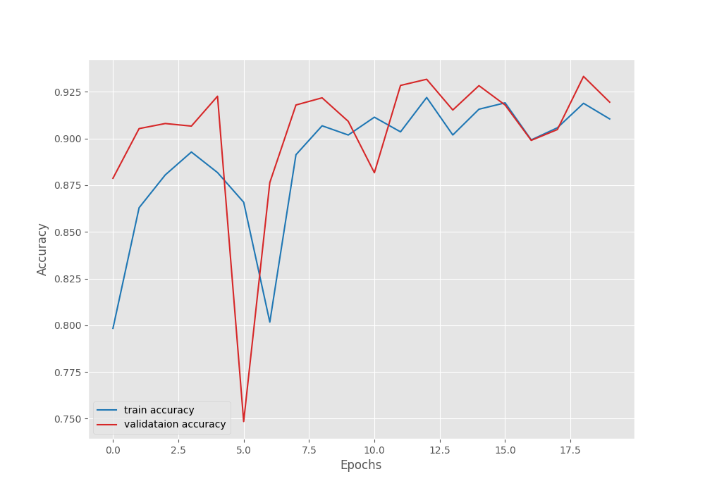
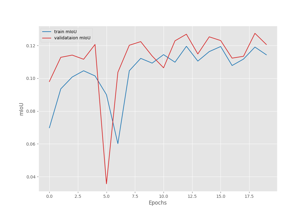
This is in contrast to what we generally expect during the fine-tuning stage. Fine-tuning is general yields better mean IoU compared to just training the segmentation head. However, we will get more insights after running inference using the trained models.
Inference using the Trained Segmentation Models
We will run inference directly on videos. The code is present in the infer_video.py file. First, we will run inference using the model where we trained the segmentation head only, then will run inference using the fine-tuned model.
Following is an example command where we run inference using the segmentation head trained model only.
python infer_video.py --input input/inference_data/videos/video_4.mp4 --imgsz 640 640 --model outputs/transfer_learning/best_model_iou.pth --save-name transfer_learn
We provide the path to the video, the image size for resizing, the model weights path and also a --save-name argument. The final argument will append a string to the resulting file name for easier recognition of the model that was used for running inference.
Let’s take a look at the results.
This is a traffic scene. Although the results look good, we can see that the segmentation maps dilate outside the object as well. Whether this is a learning issue or not can only be inferred after running inference using the completely fine-tuned model.
python infer_video.py --input input/inference_data/videos/video_4.mp4 --imgsz 640 640 --model outputs/fine_tuning/best_model_iou.pth --save-name fine_tuned
This time, we just change the path to the fine tuned model and the string appended to the resulting file name.
The dilation of the segmentation maps is much less in this case. This shows that fine-tuning the entire model may be helping.
However, let’s take a look at another pair of results before jumping to a conclusion.
Inference using segmentation head trained model only.
Inference using the completely fine-tuned model.
This time also, although not perfect the results of the completely fine-tuned DINOv2 model look much better.
Key Takeaways from DINOv2 Multi-Class Segmentation Experiments
Here are some points that we observed from the above experiments:
- We can make a general guess here that fine-tuning the entire DINOv2 model in the case of multi-class segmentation helps to achieve better segmentation maps.
- However, we could not figure out why the mean IoU was lower in the case of fine-tuning. That would require further analysis.
- We still did not achieve excellent results. The Pascal VOC dataset does not contain enough samples to train a robust model. Instead, we should pretrain the segmentation on the COCO dataset to build a robust model. We will do this in a future article.
Summary and Conclusion
In this article, we conducted fine-tuning and transfer learning experiments using DINOv2 for multi-class semantic segmentation. After training, we analyzed the results, ran inference, and discussed the key takeaways. I hope that this article was worth your time.
If you have any questions, thoughts, or suggestions, please leave them in the comment section. I will surely address them.
You can contact me using the Contact section. You can also find me on LinkedIn, and X.

I’m interested in running the code to understand. May I know how to download the code?
Hello Ishabi. You can download the code from the Download button section in the article. If that button is not responding at the moment, please try disabling ad blocker or DuckDuckGo if you have them enabled. They tend to block the download API.
Thank you for your great work.
Is it possible to make transfer learning works in segmentation task using mask2former head?
Hello. I have not tried DINOv2 backbone with Mask2Former head. However, I do have articles using Mask2Former if that helps you.
https://debuggercafe.com/fine-tuning-mask2former/
https://debuggercafe.com/multi-class-segmentation-using-mask2former/