
VLMs (Vision Language Models) are powerful AI architectures. Today, we use them for image captioning, scene understanding, and complex mathematical tasks. Large and proprietary models such as ChatGPT, Claude, and Gemini excel at tasks like converting equation images to raw LaTeX equations. However, smaller open-source models like Llama 3.2 Vision struggle, especially in 4-bit quantized format. In this article, we will tackle this use case. We will be fine-tuning Llama 3.2 Vision to convert mathematical equation images to raw LaTeX equations.
The primary aim of this article is to go through the fine-tuning process of Llama 3.2 Vision using the Unsloth library. At the same time, training it on an equation image to LaTeX equation dataset caters to a useful case.
What will we cover while training Llama 3.2 Vision?
- Exploring the LaTeX OCR dataset from Unsloth on Hugging Face.
- Loading the model and preparing the dataset in Jupyter Notebook.
- Fine-tuning the model on a subset of the dataset.
- Creating a Gradio application to easily instruct the model to generate LaTeX equations by uploading equation images.
In the previous article, while running inference, we observed how the model struggled to output raw LaTeX equations from the images. Here, we fix the issues and inconsistencies while laying out the process of data preparation, training, and inference.
The LaTeX OCR Dataset
We will use the LaTeX OCR dataset by Unsloth from Hugging Face to train the Llama VLM. We will use the Datasets library to load the model.
Let’s investigate the dataset a bit further.
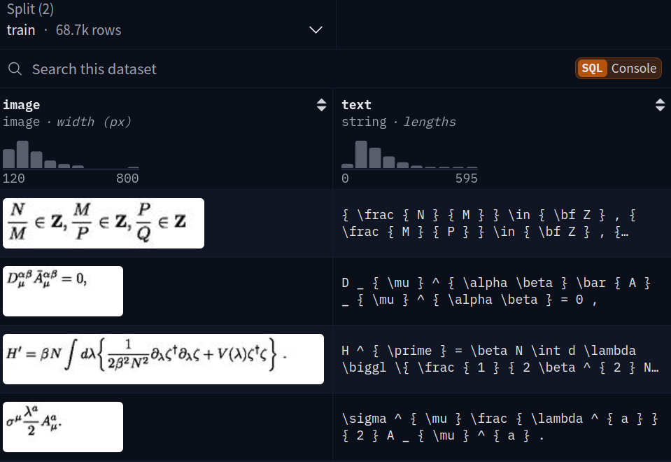
The dataset contains around 68700 training and 7600 validation samples. Each sample consists of an image and its corresponding text equation pair.
Figure 2 shows how the dataset is structured. As VLM training can be resource-intensive and costly (even in QLoRA format), we will train the Llama 3.2 Vision on a small subset of the dataset.
Directory Structure
The following is the directory structure of the project.
├── input
│   ├── image_1.png
│   ├── image_2_simple.png
│   └── image_3.png
├── outputs
│   ├── checkpoint-600
│   └── checkpoint-750
├── app.py
└── llama_3_2_vision_image2latex.ipynb
- The
inputdirectory contains the inference images that we will use to test the model after training. - The
outputsdirectory contains the trained checkpoints. - We have a Jupyter Notebook that we will use to fine-tune the model. The
app.pyscript contains the code for creating a Gradio application to chat with the trained model.
The Download Code section provides a compressed file with the input images, the Jupyter Notebook, and the Gradio application.
Download Code
Installing Requirements
- Create an Anaconda environment and install Unsloth along with other dependencies
conda create --name unsloth_env \
    python=3.11 \
    pytorch-cuda=12.1 \
    pytorch cudatoolkit xformers -c pytorch -c nvidia -c xformers \
    -y
Activate the environment.
conda activate unsloth_env
Install Unsloth and Hugging Face libraries.
pip install "unsloth[colab-new] @ git+https://github.com/unslothai/unsloth.git"
pip install --no-deps trl peft accelerate bitsandbytes
- Install Gradio
pip install gradio
That’s all the setup we need for now.
Fine-Tuning Llama 3.2 Vision for Image-to-LaTeX Equation Generation
Let’s jump right into the code without any delay.
If you wish to run inference and create a Gradio application using the pretrained model, you can visit the previous post where we discussed the Llama 3.2 Vision model. We covered its architecture and also tested it on several images.
All the code in this section is part of the llama_3_2_vision_image2latex.ipynb file.
Necessary Imports
We need the following libraries and modules while training the model.
from unsloth import FastVisionModel
from tqdm import tqdm
from transformers import TextStreamer
from unsloth import is_bf16_supported
from unsloth.trainer import UnslothVisionDataCollator
from trl import SFTTrainer, SFTConfig
from datasets import load_dataset

import matplotlib.pyplot as plt
import torch
We need the FastVisionModel class to load the Llama 3.2 Vision model.
Load the Model and the Tokenizer
The following code block loads the model in 4-bit quantized format.
model, tokenizer = FastVisionModel.from_pretrained(
    'unsloth/Llama-3.2-11B-Vision-Instruct',
    load_in_4bit=True,
    use_gradient_checkpointing='unsloth', # True or "unsloth" for long context
)
We are using the Unsloth gradient checkpointing for long context training. However, all of our prompts are small. This will become useful when training for longer caption generation.
Now, let’s prepare the model for PEFT (Parameter Efficient Fine-Tuning).
model = FastVisionModel.get_peft_model(
    model,
    finetune_vision_layers=True, # False if not finetuning vision layers
    finetune_language_layers=True, # False if not finetuning language layers
    finetune_attention_modules=True, # False if not finetuning attention layers
    finetune_mlp_modules=True, # False if not finetuning MLP layers

    r=16,           # The larger, the higher the accuracy, but might overfit
    lora_alpha=16,  # Recommended alpha == r at least
    lora_dropout=0,
    bias='none',
    random_state=3407,
    use_rslora=False,  # We support rank stabilized LoRA
    loftq_config=None, # And LoftQ
    # target_modules="all-linear", # Optional now! Can specify a list if needed
)
We are using the default arguments as suggested by the official Unsloth notebooks. They give good results out of the box. Of course, we can tinker around, however, we can start the initial training with the predefined settings.
One point to note here is that the above settings are particularly for training a VLM. They will change when fine-tuning an LLM.
Loading the Image-to-LaTeX Dataset
Loading the dataset is simple as it is already available on Hugging Face.
dataset_train = load_dataset('unsloth/LaTeX_OCR', split='train[:3000]')
dataset_test = load_dataset('unsloth/LaTeX_OCR', split='test[:500]')
We are using just 3000 samples for training and 500 samples for validation. We will be training the model on a 24GB NVIDIA L4 GPU. If you have a good hardware setup and more compute at your disposal, then you can try fine-tuning on the entire set. It will surely give better results.
We can also visualize a few samples and their corresponding equations from the training and test sets.
train_image = dataset_train[0]['image']
plt.imshow(train_image)
print(dataset_train[0]['text'])
The above code blocks give the following image and equation as outputs respectively.
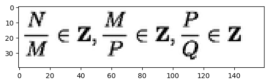
Equation:
{ \frac { N } { M } } \in { \bf Z } , { \frac { M } { P } } \in { \bf Z } , { \frac { P } { Q } } \in { \bf Z }
Creating Instruction Prompt
Before we can train the mode, we need to format the instruction prompt, that is, modify the chat template according to our use case.
instruction = 'Convert the equation images to LaTeX equations.'

def convert_to_conversation(sample):
    conversation = [
        { 'role': 'user',
          'content' : [
            {'type' : 'text',  'text'  : instruction},
            {'type' : 'image', 'image' : sample['image']} ]
        },
        { 'role' : 'assistant',
          'content' : [
            {'type' : 'text',  'text'  : sample['text']} ]
        },
    ]
    return { 'messages' : conversation }
We will call the convert_to_conversation while mapping each of the sample images and equations to create the final dataset. As we can see, we just modified the user text instruction (the user prompt), and the rest of the template remains almost unmodified.
You can learn more about chat templates and their formats in our article about the introduction to Unsloth.
The next code block maps the datasets to the above functions.
converted_dataset_train = [
    convert_to_conversation(sample) \
    for sample in tqdm(dataset_train, total=len(dataset_train))
]

converted_dataset_test = [
    convert_to_conversation(sample)
    for sample in tqdm(dataset_test, total=len(dataset_test))
]

print(converted_dataset_train[0])
Printing one of the samples gives the following output.
{
   "messages":[
      {
         "role":"user",
         "content":[
            {
               "type":"text",
               "text":"Convert the equation images to LaTeX equations."
            },
            {
               "type":"image",
               "image":<PIL.PngImagePlugin.PngImageFile image mode=RGB size=160x40 at 0x7F3EE9204430>
            }
         ]
      },
      {
         "role":"assistant",
         "content":[
            {
               "type":"text",
               "text":"{ \\frac { N } { M } } \\in { \\bf Z } , { \\frac { M } { P } } \\in { \\bf Z } , { \\frac { P } { Q } } \\in { \\bf Z }"
            }
         ]
      }
   ]
}
Internally, all the images are converted to PIL image and the model has to respond with the LaTeX equation.
Training the Model
To train the model, we need to enable training in Unsloth and define our SFTTrainer and its corresponding configurations.
FastVisionModel.for_training(model) # Enable for training!

trainer = SFTTrainer(
    model=model,
    tokenizer=tokenizer,
    data_collator=UnslothVisionDataCollator(model, tokenizer), # Must use!
    train_dataset=converted_dataset_train,
    eval_dataset=converted_dataset_test,
    args=SFTConfig(
        per_device_train_batch_size=4,
        per_device_eval_batch_size=4,
        gradient_accumulation_steps=1,
        warmup_steps=10,
        # max_steps=800,
        num_train_epochs=1, # For full training runs over the dataset.
        learning_rate=2e-4,
        fp16=not is_bf16_supported(),
        bf16=is_bf16_supported(),
        logging_steps=200,
        eval_strategy='steps',
        eval_steps=200,
        save_strategy='steps',
        save_steps=200,
        save_total_limit=2,
        optim='adamw_8bit',
        weight_decay=0.01,
        lr_scheduler_type='linear',
        seed=3407,
        output_dir='outputs',
        report_to='none',     # For Weights and Biases
        load_best_model_at_end=True,
        remove_unused_columns=False,
        dataset_text_field='',
        dataset_kwargs={'skip_prepare_dataset': True},
        dataset_num_proc=8,
        max_seq_length=2048,
        dataloader_num_workers=8
    ),
)
We have a training and evaluation batch size of 4 and are training for just 1 epoch. You can play around with the batch sizes, number of epochs to train for, and the dataloader workers depending on the hardware that you have.
Once the trainer object is initialized, we can use it to load samples from the dataloader.
dataloader = trainer.get_train_dataloader()
for i, sample in enumerate(dataloader):
    print(tokenizer.decode(sample['input_ids'][0]))
    print('#'*50)
    if i == 5:
        break
The above gives the following output.
<|begin_of_text|><|begin_of_text|><|start_header_id|>user<|end_header_id|>

Convert the equation images to LaTeX equations.<|image|><|eot_id|><|start_header_id|>assistant<|end_header_id|>

d s ^ { 2 } = - e ^ { 2 U } d t ^ { 2 } + e ^ { - 2 U } d \vec { x } ^ { 2 } \,<|eot_id|><|finetune_right_pad_id|><|finetune_right_pad_id|><|finetune_right_pad_id|>
##################################################
.
.
.
<|begin_of_text|><|begin_of_text|><|start_header_id|>user<|end_header_id|>

Convert the equation images to LaTeX equations.<|image|><|eot_id|><|start_header_id|>assistant<|end_header_id|>

q _ { j } ( x _ { 0 } ) = A _ { j + 1 }, \quad q _ { j } ^ { \prime } ( x _ { 0 } ) = B _ { j + 1 }, \quad j = 0, 1, \ldots, n - 1.<|eot_id|><|finetune_right_pad_id|><|finetune_right_pad_id|><|finetune_right_pad_id|><|finetune_right_pad_id|><|finetune_right_pad_id|><|finetune_right_pad_id|><|finetune_right_pad_id|><|finetune_right_pad_id|>
##################################################
This gives us a better idea of how the samples are modified internally, the handling of the chat templates, special tokens, and padding.
Finally, we can start the training process. The training was done on a 24 GB NVIDIA L4 GPU. It consumed around 12.5GB of VRAM and took 1 hour and 50 minutes to complete the run.
trainer_stats = trainer.train()
Following are the logs from training.
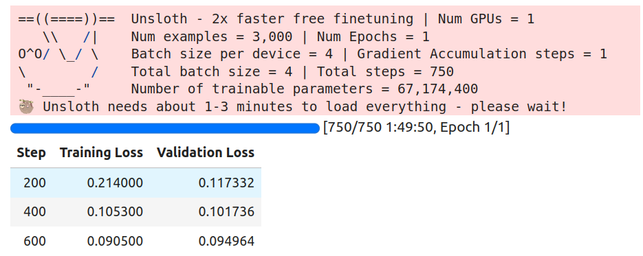
The loss kept reducing till the end. We will use the last saved checkpoint for inference when creating the Gradio application.
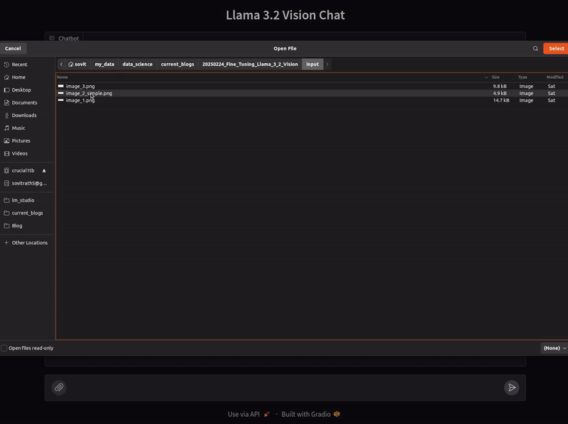
Gradio Application for Uploading Images to Convert to LaTeX
In this section, we will create the Gradio application. The code is almost the same as the previous article. We just need to change the checkpoint path to the fine-tuned checkpoint directory.
The app.py script contains all the code. We will go over the code with minimal explanation in this section. I highly recommend going through the previous article to get a detailed explanation.
Import Statements, Loading the Model, Tokenizer, and Computation Device
The following code block imports all the necessary packages, and initializes the computation device, the model, and the tokenizer. Along with that we also initialize the TextIteratorStreamer for streaming the output to the Gradio output text box.
from unsloth import FastVisionModel
from transformers import TextIteratorStreamer
from PIL import Image

import threading
import torch
import gradio as gr

device = torch.device('cuda' if torch.cuda.is_available() else 'cpu')

model, tokenizer = FastVisionModel.from_pretrained(
    model_name='outputs/checkpoint-750',
    load_in_4bit=True
)

streamer = TextIteratorStreamer(
    tokenizer, skip_prompt=True, skip_special_tokens=True
)
The model_name argument in the from_pretrained method is the local checkpoint path instead of the Hugging Face tag. Furthermore, we are loading the model in 4bit for reduced VRAM consumption.
Function to Process Images and Instructions
The following describe_image function accepts a user input that contains the text prompt and the path to the uploaded image file.
def describe_image(user_input, history):
    print(user_input)
    messages = [
        {'role': 'user', 'content': [
            {'type': 'image'},
            {'type': 'text', 'text': user_input['text']}
        ]}
    ]

    input_text = tokenizer.apply_chat_template(messages, add_generation_prompt=True)

    inputs = tokenizer(
        Image.open(user_input['files'][0]),
        input_text,
        add_special_tokens=False,
        return_tensors='pt',
    ).to(device)

    generate_kwargs = dict(
        **inputs,
        streamer=streamer,
        max_new_tokens=1024,
        use_cache=True,
        temperature=1.5,
        min_p=0.1
    )

    thread = threading.Thread(
        target=model.generate,
        kwargs=generate_kwargs
    )

    thread.start()

    outputs = []
    for new_token in streamer:
        outputs.append(new_token)
        final_output = ''.join(outputs)

        yield final_output
It tokenizes the images and text prompt, forward passes them through the model, and streams the output tokens to the text box.
Main Block
Finally, we have the main block for creating the chat interface and launching the app.
def main():
    iface = gr.ChatInterface(
        fn=describe_image,
        multimodal=True,
        title='Llama 3.2 Vision Chat',
    )

    iface.launch(share=True)

if __name__ == '__main__':
    main()
We can launch the application by executing the script.
python app.py
Analyzing Results
Let’s discuss the results by uploading a few LaTeX equation images to the application and analyzing the raw LaTeX equations.
We can start with a straightforward single-line equation.
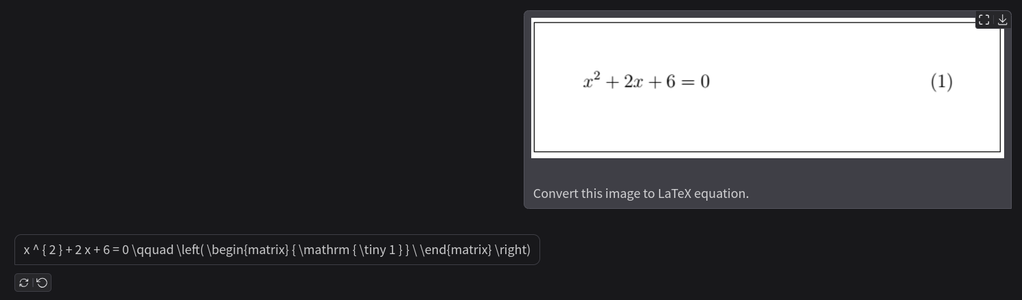
The above figure shows a single-line equation image and the response from the model is correct as well. We can easily verify the response by pasting the generated equation in the LaTeX2PNG (latex2png.com) website.
This is what we get when rendered.

The model correctly gives the LaTeX equation along with the equation number.
Now, let us try a difficult multi-line equation.
To be sure, the following is the output from LaTeX2PNG website.
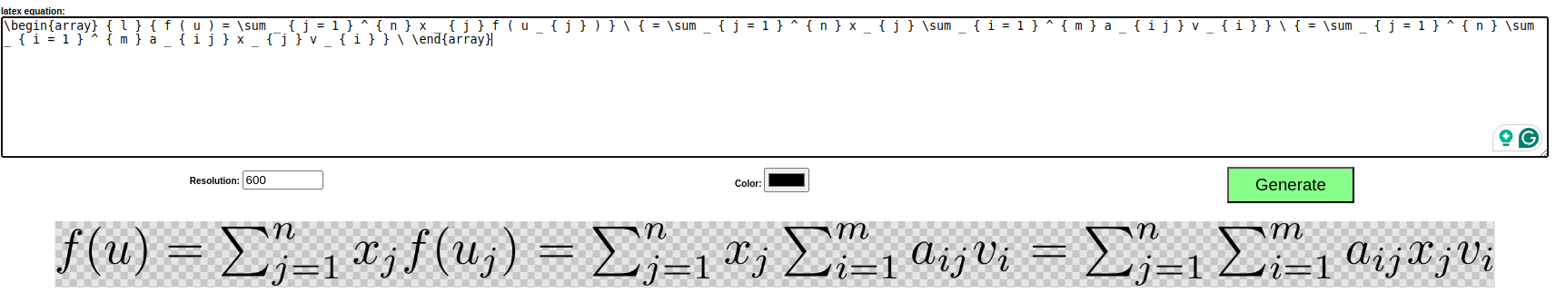
The result is interesting. Although the model predicted the equation as a single line one, because each line precedes the other by an equal sign, the result from the model is still correct. However, this may not be an ideal behavior in production use cases.
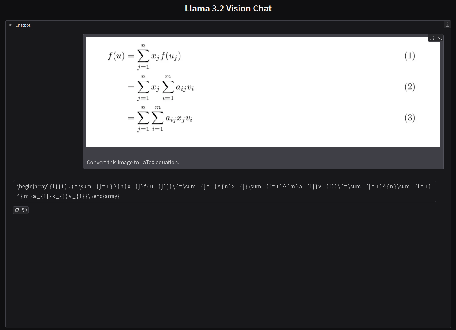
Let’s try another multi-line equation where each line is independent from the other.
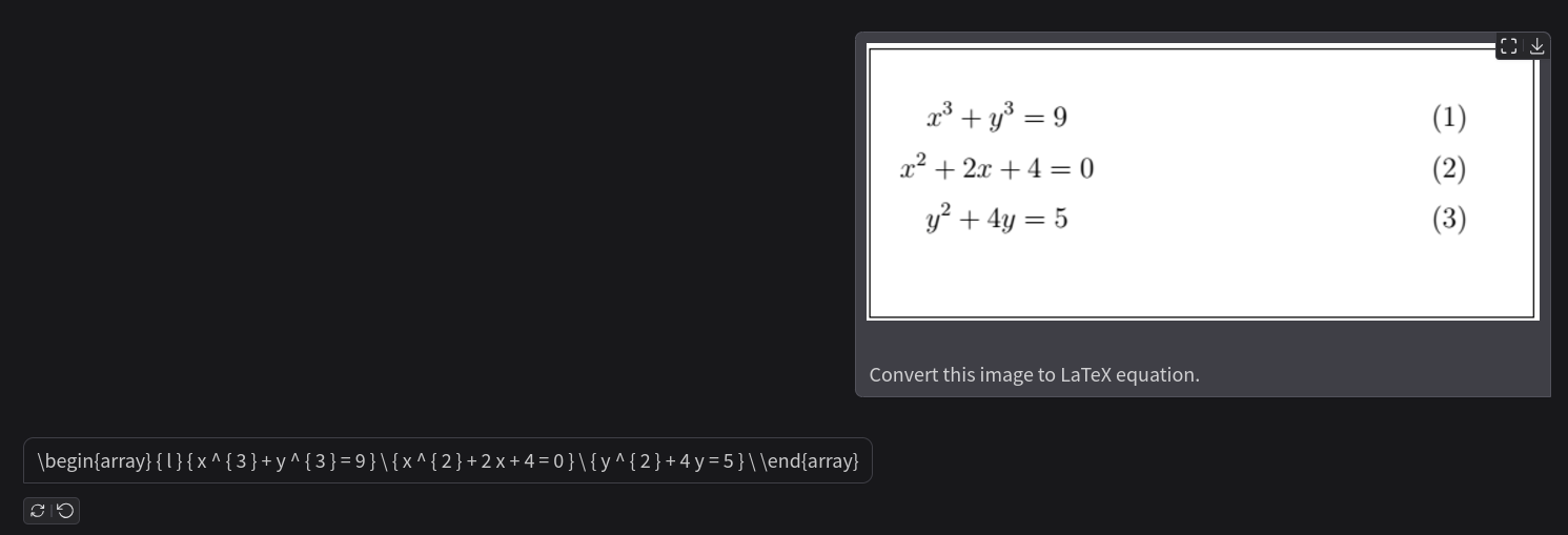
Following is the out from LaTeX2PNG.
We get the issue here. The model has predicted all the equations correctly but on a single line. In this case, however, the result becomes wrong.
Key Takeaways
Here are some takeaways from the above training run and observations.
- After training, the model is consistently predicting the equations correctly including the beginning and ending of the equations.
- However, it is struggling with multi-line equations and predicting them in a single line.
- We can correct the above behavior with more training. But the dataset we are using does not contain many multi-line equations, so, we need additional data to fix this.
Summary and Conclusion
In this article, we fine-tuned the Llama 3.2 Vision model for rendering LaTeX equations from images of LaTeX equations. We discussed the dataset, its preparation, the creation of the custom instruction template, training, and inference. During inference, we analyzed the correct and incorrect results, further discussing on how to improve the performance. I hope this article was worth your time.
If you have any questions, thoughts, or suggestions, please leave them in the comment section. I will surely address them.
You can contact me using the Contact section. You can also find me on LinkedIn, and Twitter.

2 thoughts on “Fine-Tuning Llama 3.2 Vision”