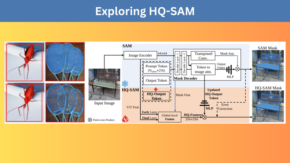
In this article, we will explore HQ-SAM (High Quality Segment Anything Model), one of the derivative works of SAM.
The Segment Anything (SAM) model by Meta revolutionized the way we think about image segmentation. Moving from a hundred thousand mask labels to more than a billion mask labels for training. From class-specific segmentation to class-agnostic segmentation, it paved the way for new possibilities. However, the very first version of SAM had its limitations. This also led the way for innovative derivative works, like HQ-SAM. This will be our primary focus in this article while absorbing as much detail as possible from the released paper.
What are we going to cover in HQ-SAM?
- What is HQ-SAM and why do we need it?
- What are the architectural changes made to the original SAM to create HQ-SAM?
- How was the dataset curated to train HQ-SAM?
- What was the training strategy?
- How does HQ-SAM stack up against the original SAM?
What is HQ-SAM and Why Do We Need It?
HQ-SAM was introduced in the paper titled Segment Anything in High Quality by Ke et al. It is a modification to the original Segment Anything Model for obtaining high quality masks when segmenting small, detailed, and intricate objects.
The original SAM model changed the way we think about object segmentation. We got a promptable segmentation model that could take user’s input via points, bounding boxes, and representation masks. This flexibility paired with the training on 1.1 billion masks, made SAM an indispensable tool in many computer vision tasks, and mainly annotation.
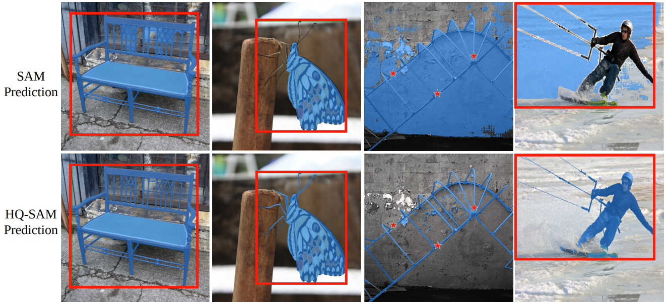
However, SAM was not good at segmenting smaller objects or those with intricate designs.
Sometimes, it missed the entire context of a prompt. For example, when the user provided a bounding for segmenting a chair, there was a high chance that it would segment the surrounding areas well.
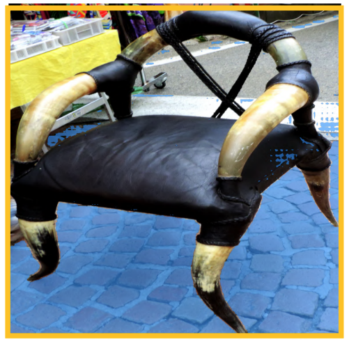
These limitations can slow down image annotation processes.
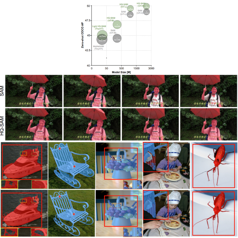
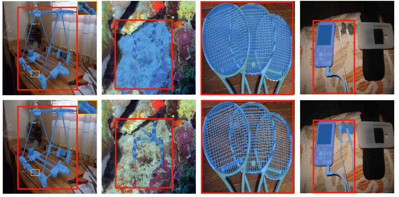
The solution came with HQ-SAM, which kept the promptable architecture of SAM intact while mitigating the above issues. HQ-SAM can predict high quality and accurate segmentation masks even for challenging images and scenes.
The above figure shows a few comparisons between SAM and HQ-SAM highlighting the latter’s capabilities. The adaptation to SAM for building HQ-SAM adds less than 0.5% parameters avoiding extra computational requirements.
What are the Architectural Changes Made to the Original SAM to Create HQ-SAM?
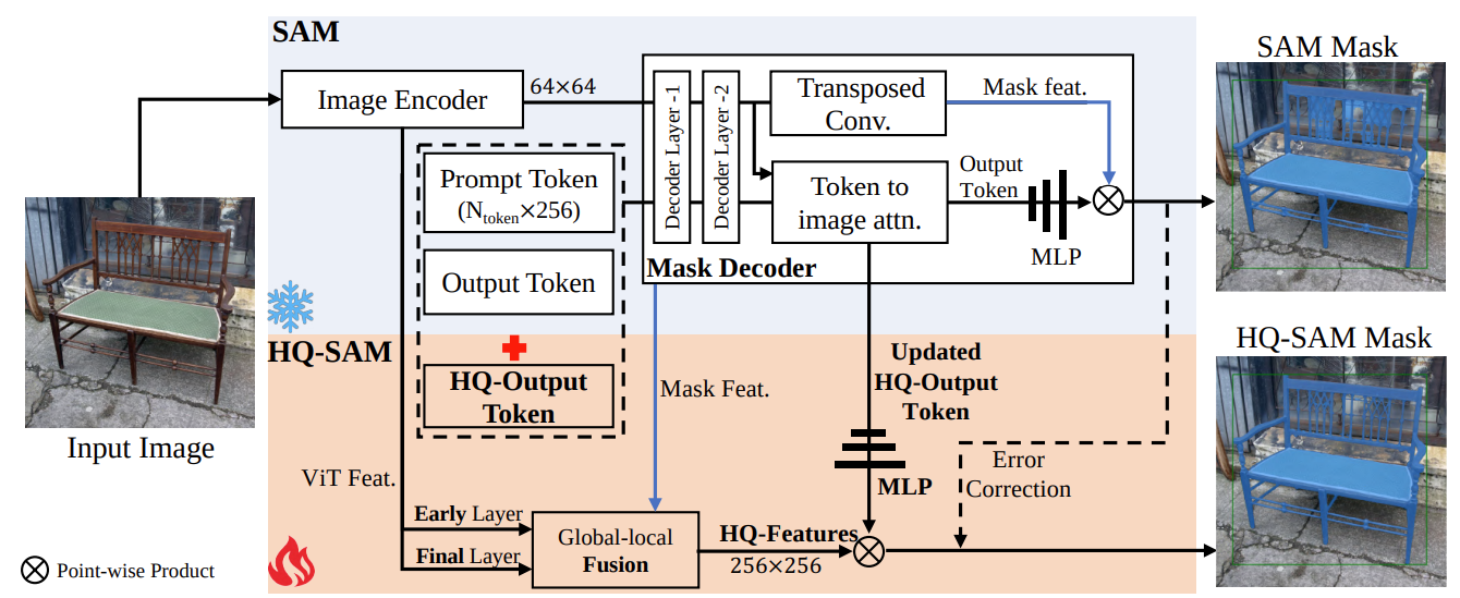
We can summarize the architectural changes in three short points:
- High quality token output: Instead of directly modifying or training the SAM decoder, the authors use the concept of an output token (similar to object query in DETR). They add a learnable High-Quality Output Token to the SAM mask decoder. This token is designed to improve mask prediction quality by leveraging both SAM’s original features and new fused features.
- Global-local feature fusion: It is difficult to predict high quality segmentation masks without the knowledge of object boundaries. However, as the image passes through several layers in a model, this boundary information is often lost. HQ-SAM employs information from three layers for this:
- Features from the early SAM ViT encoder layers which preserves the local and boundary details of the images.
- The feature from the final SAM ViT layer that preserves the global features.
- And the feature from SAM’s mask decoder layer.
- Minimal parameter addition: All of this adds only 0.5% of the original SAM model which does not make the new architecture computationally expensive.
I highly recommend going through the paper sections 3.2.1 and 3.2.2 to get the numerical details of the feature fusion step. The authors lay out the process in a clear manner and mention the layers that are used for fusion.
How was the Dataset Curated to Train HQ-SAM?
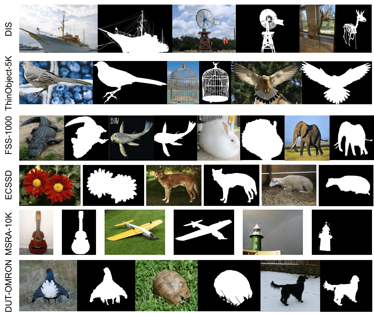
As SAM was already pretrained on SA-1B dataset, further fine-tuning on the same dataset does not yield better results. Instead, the authors curate HQSeg-44K, a dataset containing more than 44000 images with extremely accurate segmentation masks.
The HQSeg-44K is a combination of six existing datasets:
- DIS
- ThinObject-5K
- FSS-1000
- ECSSD
- MSRA-10K
- DUT-OMRON
All of the above contain extremely accurate mask annotations which is perfect for training a model like HQ-SAM. The final dataset contains more than 1000 diverse classes of objects.
This dataset overcomes one of the major limitations of SA-1B, the lack of fine-grained segmentation masks for training. Furthermore, the new dataset’s small size allows for rapid training experimentation.
What was the Strategy and Setup for Training HQ-SAM?
During training, the new HQ-SAM layers are learnable while keeping the original SAM layers frozen. This makes the output token, the three MLP layers, and three convolution operations learnable in the proposed HQ-SAM architecture.
The following are the hyperparameters for the training process:
- Learning rate: 0.001
- Number of epochs: 12 with the learning rate dropping after 10 epochs
As the dataset contains only around 44000 images, training HQ-SAM took only 4 hours on 8 RTX-3090 GPUs with a batch size of 32.
The authors also use large-scale jittering as an augmentation step to make the model learn more fine-grained features in objects of varying scales.
Comparison Against SAM
In this section, we will cover the various comparisons the authors make between SAM and HQ-SAM.
Training and Inference Compute
Let’s start with the simplest comparison, the resources required for training and inference on each model.
The above table shows a stark contrast between the resource requirements of both models. On the one hand, the original SAM model requires 128 A100 GPUs while running at 5 FPS during inference. On the other hand, HQ-SAM while keeping the inference requirements the same, reduces the training compute drastically by having only 5 million training parameters with a batch size of 32. All this while taking only 4 hours to train.
COCO Segmentation Results
Following from here, we will cover the general experimental results as mentioned by the authors.
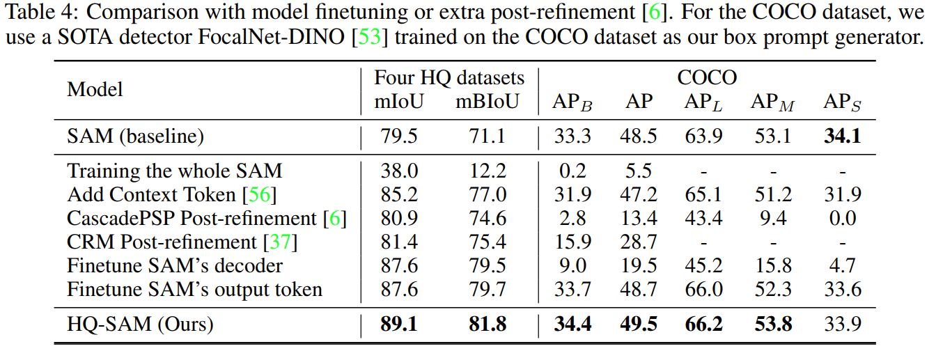
The next table shows the benchmarks between SAM and HQ-SAM on the COCO dataset.
In the above figure, mIoU is mask IoU and mBIoU is border IoU. It is clear that the new model is ahead of SAM in both metrics. In fact, the authors also go on to show that retraining the entire mask decoder of SAM does not yield the same result as their new HQ-SAM architecture. For the above experiments, a SOTA FocalNet-DINO detector was used as the bounding box prompt generator.
Visual Results
Following are some of the visual results provided in the paper.
In Figure 10, we can see that the HQ-SAM model is robust to small mistakes in the bounding box prompts when the box does not cover the entire object.
Summary and Conclusion
In this article, we covered the HQ-SAM architecture in brief. We started with the need for HQ-SAM, its architecture, training, and experimental results. In conclusion, the final HQ-SAM model gives superior segmentation masks while keeping the inference requirements the same as SAM. I hope that this article was worth your time.
If you have any doubts, thoughts, or suggestions, please leave them in the comment section. I will surely address them.
You can contact me using the Contact section. You can also find me on LinkedIn, and Twitter.

