

This article is a continuation of the DINOv3 series. This is an incremental post on the lines of object detection using DINOv3 backbone. While in the last article, we used the SSD head for object detection with DINOv3, in this one, we will improve upon it by adding the capability for the RetinaNet head as well. We will carry out both training and inference with DINOv3 with RetinaNet head for object detection.

We will continue using the DINOv3 Stack project and borrow most of the setup and dataset discussion steps from the last article. I highly recommend going through the previous article, where we discussed DINOv3 object detection with SSD head.
We will discuss the following topics here while covering DINOv3 RetinaNet object detection:
- Brief discussion of the Pascal VOC dataset and the project setup.
- Detailed discussion of the model architecture and training code modifications to support both SSD and RetinaNet heads.
- Training and inference discussion.
- Key takeaways with steps for improvement and concluding remarks.
The Pascal VOC Detection Dataset
We have discussed the Pascal VOC object detection dataset in detail in the last article.
In short, it contains ~16500 training and ~5000 validation samples.
We will use the dataset present on Kaggle here. It follows the following structure after downloading and extracting.
├── voc_07_12
│   └── voc_xml_dataset
│       ├── train
│       │   ├── images  [16551 entries exceeds filelimit, not opening dir]
│       │   └── labels  [16551 entries exceeds filelimit, not opening dir]
│       ├── valid
│       │   ├── images  [4952 entries exceeds filelimit, not opening dir]
│       │   └── labels  [4952 entries exceeds filelimit, not opening dir]
│       └── README.txt
└── readme.txt
The annotations are present in XML format.
Project Directory Structure
Following is the project directory structure. It is almost the same as we had in the last article, as we are dealing with the same DINOv3 Stack codebase from GitHub.
├── classification_configs
│   └── leaf_disease.yaml
├── dinov3
│   ├── dinov3
│   │   ├── checkpointer
│   │   ├── configs
│   │   ├── data
│   │   ...
│   │   └── __init__.py
│   ├── __pycache__
│   │   └── hubconf.cpython-312.pyc
│   ...
│   ├── requirements-dev.txt
│   ├── requirements.txt
│   └── setup.py
├── input
│   ├── voc_07_12
│   │   └── voc_xml_dataset
│   └── readme.txt
├── outputs
│   └── img_det
│       ├── best_model.pth
│       ├── last_model.pth
│       ├── map.png
│       └── train_loss.png
├── segmentation_configs
│   ├── person.yaml
│   └── voc.yaml
├── src
│   ├── detection
│   │   ├── __pycache__
│   │   ├── analyze_dataset.py
│   │   ├── config.py
│   │   ├── custom_utils.py
│   │   ├── datasets.py
│   │   ├── eval.py
│   │   └── model.py
│   ├── img_cls
│   │   ├── datasets.py
│   │   ├── __init__.py
│   │   ├── model.py
│   │   └── utils.py
│   ├── img_seg
│   │   ├── datasets.py
│   │   ├── engine.py
│   │   ├── __init__.py
│   │   ├── metrics.py
│   │   ├── model.py
│   │   └── utils.py
│   └── utils
│       ├── __pycache__
│       └── common.py
├── weights
│   └── dinov3_convnext_tiny_pretrain_lvd1689m-21b726bb.pth
├── infer_classifier.py
├── infer_det_image.py
├── infer_det_video.py
├── infer_seg_image.py
├── infer_seg_video.py
├── License
├── NOTES.md
├── Outputs.md
├── README.md
├── requirements.txt
├── train_classifier.py
├── train_detection.py
└── train_segmentation.py
- We have the training and inference scripts for detection in the parent project directory, and the engine and utility modules inside
src/detection. - The dataset that we downloaded above is present in the
inputdirectory. - The
outputsdirectory contains all the training and inference data. dinov3is the cloned official DINOv3 repository.
The entire codebase, along with trained weights and inference data is available via the download section. You can directly run the inference. If you wish to run the training, please download the dataset and arrange it in the above structure.
Download Code
Setup and Managing Dependencies
I recommend following the previous article for setup, as it lays out the steps in detail, and they remain the same here. The major steps are cloning the DINOv3 repository and creating the .env file with the correct path credentials.
DINOv3 Object Detection with RetinaNet Head
Let’s jump into the coding section. We will only cover the important parts of the code that differ from the previous article. These include the modeling section and a bit of the training script.
DINOv3 RetinaNet Model
The code that we are discussing here is present in the src/detection/model.py file.
The following block contains the entire code.
import torch
import torch.nn as nn
import os

from torchvision.models.detection.ssd import (
    SSD,
    DefaultBoxGenerator,
    SSDHead
)
from torchvision.models.detection.retinanet import (
    RetinaNet, RetinaNetHead, AnchorGenerator
)

def load_model(weights: str=None, model_name: str=None, repo_dir: str=None):
    if weights is not None:
        print('Loading pretrained backbone weights from: ', weights)
        model = torch.hub.load(
            repo_dir,
            model_name,
            source='local',
            weights=weights
        )
    else:
        print('No pretrained weights path given. Loading with random weights.')
        model = torch.hub.load(
            repo_dir,
            model_name,
            source='local'
        )

    return model

class Dinov3Backbone(nn.Module):
    def __init__(self,
        weights: str=None,
        model_name: str=None,
        repo_dir: str=None,
        fine_tune: bool=False
    ):
        super(Dinov3Backbone, self).__init__()

        self.model_name = model_name

        self.backbone_model = load_model(
            weights=weights, model_name=model_name, repo_dir=repo_dir
        )

        if fine_tune:
            for name, param in self.backbone_model.named_parameters():
                param.requires_grad = True
        else:
            for name, param in self.backbone_model.named_parameters():
                param.requires_grad = False

    def forward(self, x):
        out = self.backbone_model.get_intermediate_layers(
            x,
            n=1,
            reshape=True,
            return_class_token=False,
            norm=True
        )[0]

        return out

def dinov3_detection(
    fine_tune: bool=False,
    num_classes: int=2,
    weights: str=None,
    model_name: str=None,
    repo_dir: str=None,
    resolution: list=[640, 640],
    nms: float=0.45,
    feature_extractor: str='last', # OR 'multi'
    head: str='ssd' # Detection head type, ssd or retinanet
):
    backbone = Dinov3Backbone(
        weights=weights,
        model_name=model_name,
        repo_dir=repo_dir,
        fine_tune=fine_tune
    )

    if head == 'ssd':
        out_channels = [backbone.backbone_model.norm.normalized_shape[0]] * 6
        anchor_generator = DefaultBoxGenerator(
            aspect_ratios=[[2], [2, 3], [2, 3], [2, 3], [2], [2]],
        )

        num_anchors = anchor_generator.num_anchors_per_location()
        det_head = SSDHead(out_channels, num_anchors, num_classes=num_classes)

        model = SSD(
            backbone=backbone,
            num_classes=num_classes,
            anchor_generator=anchor_generator,
            size=resolution,
            head=det_head,
            nms_thresh=nms
        )

    elif head == 'retinanet':
        backbone.out_channels = backbone.backbone_model.norm.normalized_shape[0]
        anchor_sizes = ((32, 64, 128, 256, 512),)
        aspect_ratios = ((0.5, 1.0, 2.0),)
        anchor_generator = AnchorGenerator(anchor_sizes, aspect_ratios)

        model = RetinaNet(
            backbone=backbone,
            num_classes=num_classes,
            anchor_generator=anchor_generator,
            min_size=resolution[0],
            max_size=resolution[1],
            # head=head,
            nms_thresh=nms
        )
In the import section, we have modules for both the SSD and the RetinaNet heads. This is because we can choose either of the two to build the detection head.
The load_model function and the Dinov3Backbone class remain the same as in the previous article.
The only change happens in the dinov3_detection function. Here, we can pass an extra head parameter now. This is a string that can be either ssd or retinanet. Then we build the model according to that.
The RetinaNet head is built from line 102. We use well-known anchor sizes and aspect ratios. These work as good defaults and are almost the same as the ones used in Torchvision models. And we have only single tuples for both, as we are not using multiple feature maps at the moment. We are extracting the last feature map from the backbone to build the detection model.
This is a very simple process to build the model at the moment. With multi-feature map, it will become slightly more sophisticated, and some parts would change.
The Training Script
The training script, that is, train_detection.py now contains an additional command line argument, --head. We can either pass ssd, or retinanet, and the default value is retinanet as the RetinaNet model gives better results compared to the SSD model at the moment.
All the training and inference experiments were carried out on a system with 10GB RTX 3080, 32GB RAM, and a 10th generation i7 processor.
Let’s start the training. We can execute the following command in a terminal within the parent project directory.
python train_detection.py \
--weight dinov3_convnext_tiny_pretrain_lvd1689m-21b726bb.pth \
--model-name dinov3_convnext_tiny \
--imgsz 640 640 \
--lr 0.0001 \
--epochs 30 \
--workers 8 \
--batch 8 \
--config detection_configs/voc.yaml \
--head retinanet
The arguments remain almost the same as in the previous article, with the exception of the --head.
Note that we are not fine-tuning the entire model here. The backbone remains frozen, and we train the RetinaNet head. This results in about 45 million trainable parameters out of the total of 72.8 million total parameters.
Here are the truncated terminal outputs.
72,885,975 total parameters.
45,065,847 training parameters.
Using AdamW (
Parameter Group 0
    amsgrad: False
    betas: (0.9, 0.999)
    capturable: False
    decoupled_weight_decay: True
    differentiable: False
    eps: 1e-08
    foreach: None
    fused: None
    lr: 0.0001
    maximize: False
    weight_decay: 0.01
) for dinov3_convnext_tiny
.
.
.
Epoch #1 train loss: 0.911
Epoch #1 [email protected]:0.95: 0.221271350979805
Epoch #1 [email protected]: 0.48972538113594055
Took 5.756 minutes for epoch 0

BEST VALIDATION mAP: 0.221271350979805

SAVING BEST MODEL FOR EPOCH: 1

SAVING PLOTS COMPLETE...
.
.
.
Epoch #28 train loss: 0.188
Epoch #28 [email protected]:0.95: 0.3981453776359558
Epoch #28 [email protected]: 0.7118459343910217
Took 5.748 minutes for epoch 27

BEST VALIDATION mAP: 0.3981453776359558

SAVING BEST MODEL FOR EPOCH: 28

SAVING PLOTS COMPLETE...
LR for next epoch: [0.0001]
.
.
.
Epoch #30 train loss: 0.183
Epoch #30 [email protected]:0.95: 0.39631354808807373
Epoch #30 [email protected]: 0.7056518793106079
Took 5.699 minutes for epoch 29
SAVING PLOTS COMPLETE...
LR for next epoch: [0.0001]
The best model was saved on epoch 28 with an mAP of 39.8%.
Let’s take a look at the mAP and loss plots.

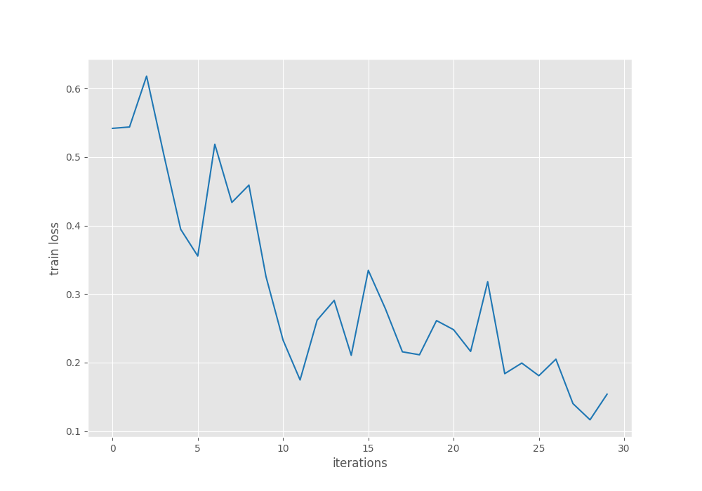
The mAP seems to have completely plateaued by the end of training. For further experiments, we can use a learning rate scheduler and train for longer to check whether that leads to an improvement or not.
For now, we will use the trained model for inference.
Inference Using the Trained DINOv3 RetinaNet Model
First, we will carry out image inference, the code for which is present in the infer_det_image.py file.
python infer_det_image.py \
--input input/inference_data/images/ \
--imgsz 640 \
--model outputs/img_det/best_model.pth \
--model-name dinov3_convnext_tiny \
--config detection_configs/voc.yaml \
--head retinanet \
--threshold 0.5
We are providing the following command line arguments:
--input: The path to the directory containing the images.--imgsz: The resolution for resizing the images. All the images will be resized to 640×640 resolution. This is the same as training.--model: This is the path to the trained weight file.--model-name: The backbone model name.--head: The detection head name.--threshold: This is the detection confidence threshold.
The following are some of the results.
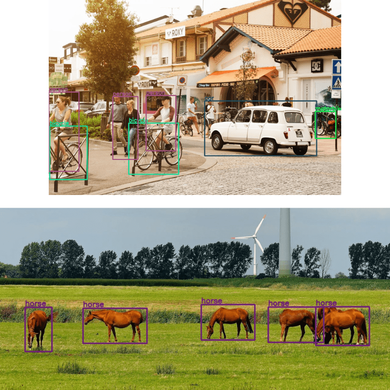
The results are good, but there is still plenty of room for improvement. Some of the people in the back are not detected, and in most cases, the bounding boxes do not enclose the object tightly. I recommend running experiments on some of your own images and checking the results.
Let’s move to video inference, whose code is present in the infer_det_video.py file.
python infer_det_video.py \
--input input/inference_data/videos/video_1.mp4 \
--imgsz 640 \
--model outputs/img_det/best_model.pth \
--model-name dinov3_convnext_tiny \
--config detection_configs/voc.yaml \
--head retinanet \
--threshold 0.6
With the exception of the script name and the confidence threshold, the other command line arguments remain the same.
Here is the resulting video output.
We can see some of the glaring issues right away. Even if the objects are not that far away, the model is unable to detect them, e.g., the second horse and the person beside the car.
Let’s take a look at another example.
This is a more crowded scene. Although the model seems to be performing well here, flickering is an issue.
One silver lining is that even for a 72 million parameter model, on an RTX 3080, we are getting almost an average of 70 FPS.
Takeaways
There is much room for improvement here.
- We are not training either the SSD or the RetinaNet models with multi-level feature maps at the moment. Doing so will surely improve the results.
- The augmentations are pretty basic, with only horizontal flipping. Adding more complex augmentations will also teach the model to handle different scenarios.
Summary and Conclusion
In this article, we discussed an incremental improvement of using the RetinaNet head for DINOv3 object detection. We discussed the model changes and analyzed the inference results. As the above-discussed points get implemented into the DINOv3 Stack codebase, more articles will be published with the improvements.
If you have any questions, thoughts, or suggestions, please leave them in the comment section. I will surely address them.
You can contact me using the Contact section. You can also find me on LinkedIn, and X.
