
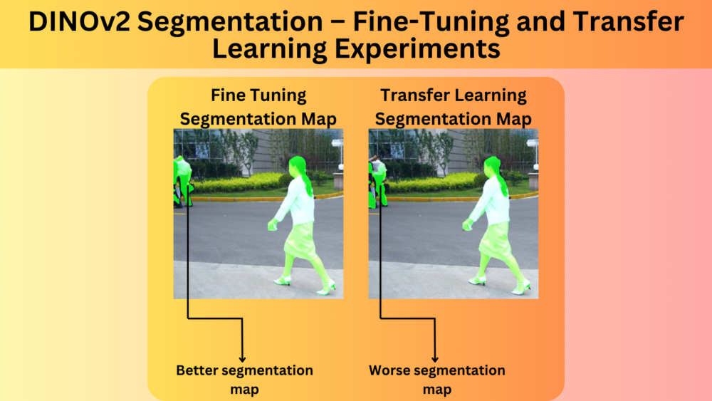
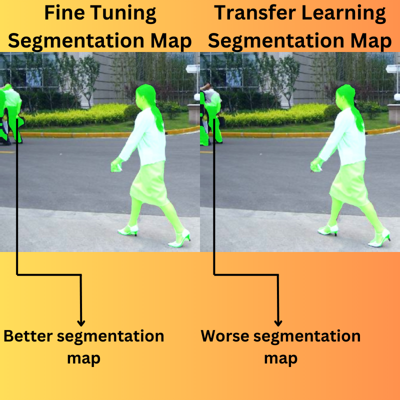
DINOv2’s SSL training leads to its learning extremely powerful image features. We can use such a trained backbone for numerous downstream tasks like image classification, image segmentation, feature matching, and object detection. In this article, we will experiment with DINOv2 segmentation for fine-tuning and transfer learning.
What are we going to cover in DINOv2 fine-tuning and transfer learning segmentation experiments?
- What are the contributions of this article?
- How do we build a simple model and training pipeline?
- How do we set up the training experiments?
- What results are we getting in each experiment?
Note: This article is a follow-up to the previous one where we started with DINOv2 semantic segmentation experiments. It will be a short article where we will focus on the modeling code and experiment results.
What Are the Contributions of This Article?
In the previous article, we trained the DINOv2 model for semantic segmentation.
We discarded the MMSegmentation requirement from the modeling pipeline that the original authors used. Furthermore, we built the model with the pixel classification head as present in the original DINOv2 codebase along with hardcoded model parameters.
This made the entire modeling pipeline complex. In this article, we will mitigate some of the issues. To this end, this article has two primary contributions:
- Simplify the modeling pipeline with a custom segmentation head.
- Run experiments for fine-tuning and transfer learning for DINOv2 segmentation.
As discussed in the previous article, this is part of a larger project and the experiments are still in the early stages. As such, we will still hardcode some of the model hyperparameters while building it.
The Person Segmentation Dataset
We will use the same person segmentation dataset that we did in the last article. Please refer to it to get more details on the dataset.
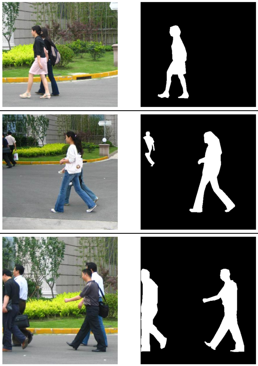
You can download the dataset from here on Kaggle.
Project Directory Structure
Let’s look at the project directory structure before running the experiments.
├── input
│   ├── inference_data
│   └── PennFudanPed
├── notebooks
│   └── visualize.ipynb
├── outputs
│   ├── fine_tuning
│   ├── transfer_learning
│   └── transfer_learning_schd
├── config.py
├── datasets.py
├── engine.py
├── infer_image.py
├── infer_video.py
├── metrics.py
├── model_config.py
├── model.py
├── requirements.txt
├── train.py
└── utils.py
We follow almost the same structure as the last article.
- The
inputsdirectory contains the dataset. - The
outputsdirectory contains the training results. - Finally, the parent project directory contains the Python files.
All the Python code files, best trained models from each training experiments, and inference data is available via the download section.
Download Code
All the necessary libraries can be installed using the requirements file.
pip install -r requirements.txt
Running Transfer Learning and Fine Tuning Segmentation Experiments using DINOv2 Backbone
In this section, we will primarily discuss all the important coding parts necessary for the experiments.
The Modified DINOv2 Segmentation Model
We will discuss the necessary changes that were made to the DINOv2 semantic segmentation model. We have simplified the modeling part quite a bit. The code that follows is present in the model.py file.
Let’s start with all the import statements.
import torch
import torch.nn as nn

from functools import partial
from collections import OrderedDict
from torchinfo import summary
from model_config import model as model_dict
Among the necessary imports, we have the model_dict from model_config.
In the last article, we downloaded the model configuration originally used as part of MMSegmentation experiments by the authors. These configuration files define the model backbone and model head along with the training parameters. However, in this article, we already use the content from those downloaded files and store them in model_config.py. We need the model_dict information only from the configuration. In fact, in the future, we can have a separate configuration file defining the hyperparameters of all the models.
Function to Load the DINOv2 Backbone
Next, we define the load_backbone function to load the DINOv2 Small backbone.
def load_backbone():
    BACKBONE_SIZE = "small" # in ("small", "base", "large" or "giant")

    backbone_archs = {
        "small": "vits14",
        "base": "vitb14",
        "large": "vitl14",
        "giant": "vitg14",
    }
    backbone_arch = backbone_archs[BACKBONE_SIZE]
    backbone_name = f"dinov2_{backbone_arch}"


    backbone_model = torch.hub.load(repo_or_dir="facebookresearch/dinov2", model=backbone_name)
    backbone_model.cuda()

    backbone_model.forward = partial(
        backbone_model.get_intermediate_layers,
        n=model_dict['backbone']['out_indices'],
        reshape=True,
    )

    return backbone_model
We define the backbone architectures and the one that we want to use. We use TorchHub to load the backbone and transfer it to the CUDA device. Then we use the same strategy as in the last article to define a partial method that will return features from 4 different layers during the forward pass.
The Linear Pixel Classifier
If you have gone through the previous blog post, you might realize that the segmentation head was complex. Here, we will simplify that using some of the code as discussed in this GitHub issue.
class LinearClassifierToken(torch.nn.Module):
    def __init__(self, in_channels, nc=1, tokenW=32, tokenH=32):
        super(LinearClassifierToken, self).__init__()
        self.in_channels = in_channels
        self.W = tokenW
        self.H = tokenH
        self.nc = nc
        self.conv = torch.nn.Conv2d(in_channels, nc, (1, 1))

    def forward(self,x):
        outputs =  self.conv(
            x.reshape(-1, self.in_channels, self.H, self.W)
        )
        return outputs
We define the LinearClassifierToken class which accepts the following parameters:
in_channels: The input channels to the final pixel classification Convolutional layer. This should be the same dimension as the output from the DINOv2 backbonenc: The number of classes in the dataset.tokenWandtokenH: We are using the DINOv2 Small Patch-14 model which creates patches of 14×14 dimension. This means that an input image of 644×644 will contain 46 patches each across the width and height. These are the tokens whose number is necessary to reshape the final output. Although the default value is 32, we will pass the correct value during initialization. For an input resolution of 644×644, the outputs will be of the shape[batch_size, in_channels, 46, 46].
The Final DINOv2 Segmentation Model
We finally combine the backbone and the segmentation head using a Sequential Ordered dictionary.
class Dinov2Segmentation(nn.Module):
    def __init__(self, fine_tune=False):
        super(Dinov2Segmentation, self).__init__()

        self.backbone_model = load_backbone()
        print(fine_tune)
        if fine_tune:
            for name, param in self.backbone_model.named_parameters():
                param.requires_grad = True
        else:
            for name, param in self.backbone_model.named_parameters():
                param.requires_grad = False

        self.decode_head = LinearClassifierToken(in_channels=1536, nc=2, tokenW=46, tokenH=46)

        self.model = nn.Sequential(OrderedDict([
            ('backbone', self.backbone_model),
            ('decode_head', self.decode_head)
        ]))

    def forward(self, x):
        features = self.model.backbone(x)

        # `features` is a tuple.
        concatenated_features = torch.cat(features, 1)

        classifier_out = self.decode_head(concatenated_features)

        return classifier_out
Note that the backbone returns a tuple of features from 4 different layers. We concatenate them in the forward pass for the best results. These features are then passed to the model’s decode_head.
Furthermore, as we will carry out both, transfer learning and fine-tuning experiments, the model class accepts a fine_tune parameter that we use to control the trainable parameters in the backbone.
This brings us to the end of the model building part of DINOv2 segmentation for fine-tuning and transfer learning experiments.
The rest of the implementation such as data set preparation, transforms, and augmentations, remains exactly the same as the previous article.
Transfer Learning Experiment for DINOv2 Segmentation
All experiments were run on a system with 10GB RTX 3080 GPU, 32GB RAM, and a 10th generation i7 CPU.
Let’s start with the transfer learning experiment. We can execute the following command in the terminal within the parent project directory.
python train.py --lr 0.0005 --batch 2 --imgsz 640 640 --epochs 65 --out-dir transfer_learning
Following are the command line arguments that we are using:
--lr: The base learning rate for the optimizer. For transfer learning, we use a learning rate of 0.0005.--batch: This defines the batch size and we use a value of 2. We use a smaller batch size because during fine-tuning, we will train all the parameters and the 10GB GPU could only allocate a batch size of 2. To keep the experimental results comparable, we use the same batch size for transfer learning as well.--imgsz: This is the resolution that the images and masks will be resized to. All samples will be resized to 640×640 resolution first and then padded with 4 pixels to make the final resolution 644×644.--epochs: The number of epochs for which the model is trained.--out-dir: The subdirectory name inside the outputs directory. We maintain a different directory for each experiment.
Following are the truncated outputs from the terminal.
=============================================================================================================================
Layer (type (var_name))                            Input Shape               Output Shape              Param #
=============================================================================================================================
Dinov2Segmentation (Dinov2Segmentation)            [1, 3, 644, 644]          [1, 2, 46, 46]            --
├─Sequential (model)                               --                        --                        --
│    └─DinoVisionTransformer (backbone)            [1, 3, 644, 644]          [1, 384, 46, 46]          526,848
│    │    └─PatchEmbed (patch_embed)               [1, 3, 644, 644]          [1, 2116, 384]            (226,176)
│    │    └─ModuleList (blocks)                    --                        --                        (21,302,784)
│    │    └─LayerNorm (norm)                       [1, 2117, 384]            [1, 2117, 384]            (768)
│    │    └─LayerNorm (norm)                       [1, 2117, 384]            [1, 2117, 384]            (recursive)
│    │    └─LayerNorm (norm)                       [1, 2117, 384]            [1, 2117, 384]            (recursive)
│    │    └─LayerNorm (norm)                       [1, 2117, 384]            [1, 2117, 384]            (recursive)
│    └─LinearClassifierToken (decode_head)         [1, 1536, 46, 46]         [1, 2, 46, 46]            3,074
│    │    └─Conv2d (conv)                          [1, 1536, 46, 46]         [1, 2, 46, 46]            3,074
=============================================================================================================================
Total params: 22,062,724
Trainable params: 6,148
Non-trainable params: 22,056,576
Total mult-adds (Units.MEGABYTES): 506.39
=============================================================================================================================
Input size (MB): 4.98
Forward/backward pass size (MB): 1047.08
Params size (MB): 86.13
Estimated Total Size (MB): 1138.19
=============================================================================================================================
EPOCH: 1
Training
100%|████████████████████| 73/73 [00:05<00:00, 13.93it/s]
Validating
100%|████████████████████| 12/12 [00:01<00:00, 10.91it/s]

Best validation loss: 0.10560639388859272

Saving best model for epoch: 1


Best validation IoU: 0.7998962055528813

Saving best model for epoch: 1

Train Epoch Loss: 0.2430, Train Epoch PixAcc: 0.8928, Train Epoch mIOU: 0.725339
Valid Epoch Loss: 0.1056, Valid Epoch PixAcc: 0.8853 Valid Epoch mIOU: 0.799896
LR for next epoch: [0.0005]
--------------------------------------------------
EPOCH: 2
Training
100%|████████████████████| 73/73 [00:04<00:00, 14.67it/s]
Validating
100%|████████████████████| 12/12 [00:01<00:00, 11.02it/s]

Best validation loss: 0.0952610798800985

Saving best model for epoch: 2


Best validation IoU: 0.8058518124519641

Saving best model for epoch: 2

Train Epoch Loss: 0.2067, Train Epoch PixAcc: 0.9144, Train Epoch mIOU: 0.777027
Valid Epoch Loss: 0.0953, Valid Epoch PixAcc: 0.8876 Valid Epoch mIOU: 0.805852
LR for next epoch: [0.0005]
--------------------------------------------------
EPOCH: 3
Training
100%|████████████████████| 73/73 [00:05<00:00, 13.75it/s]
Validating
100%|████████████████████| 12/12 [00:01<00:00, 10.91it/s]

Best validation loss: 0.08329576129714648

Saving best model for epoch: 3


Best validation IoU: 0.8209524461889638

Saving best model for epoch: 3

Train Epoch Loss: 0.2058, Train Epoch PixAcc: 0.9150, Train Epoch mIOU: 0.779935
Valid Epoch Loss: 0.0833, Valid Epoch PixAcc: 0.8926 Valid Epoch mIOU: 0.820952
LR for next epoch: [0.0005]
--------------------------------------------------
.
.
.
EPOCH: 41
Training
100%|████████████████████| 73/73 [00:06<00:00, 12.16it/s]
Validating
100%|████████████████████| 12/12 [00:01<00:00, 10.49it/s]

Best validation loss: 0.06764321448281407

Saving best model for epoch: 41


Best validation IoU: 0.8373048613831366

Saving best model for epoch: 41

Train Epoch Loss: 0.1349, Train Epoch PixAcc: 0.9311, Train Epoch mIOU: 0.807703
Valid Epoch Loss: 0.0676, Valid Epoch PixAcc: 0.8978 Valid Epoch mIOU: 0.837305
LR for next epoch: [0.0005]
--------------------------------------------------
.
.
.
EPOCH: 65
Training
100%|████████████████████| 73/73 [00:05<00:00, 13.81it/s]
Validating
100%|████████████████████| 12/12 [00:01<00:00, 11.06it/s]

Best validation loss: 0.06727483573680122

Saving best model for epoch: 65

Train Epoch Loss: 0.1856, Train Epoch PixAcc: 0.9277, Train Epoch mIOU: 0.806646
Valid Epoch Loss: 0.0673, Valid Epoch PixAcc: 0.8975 Valid Epoch mIOU: 0.836716
LR for next epoch: [0.0005]
--------------------------------------------------
TRAINING COMPLETE
The model reached the best mean IoU of 83.7% on epoch 41. For a better analysis, let’s examine the loss, accuracy, and mean IoU graphs.
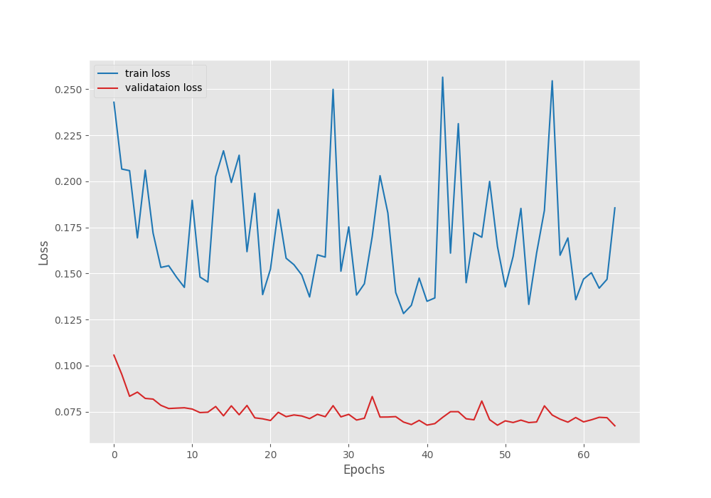
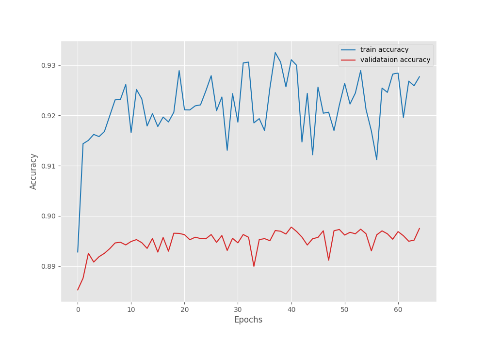
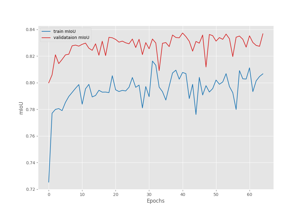
We can see that the training is slightly unstable. The most probable explanation is that we can start with a lower learning rate. That might make the learning more stable, however, there is a minimal chance that it will lead to higher IoU.
Another interesting point to note here is that the mean IoU reached more than 82% by the end of epoch 3. This shows that the DINOv2 backbone has already learned powerful features which leads to faster training of the segmentation head.
Fine-Tuning Experiment for DINOv2 Segmentation
Now, let us carry out the fine-tuning experiment where we will train the backbone as well as the segmentation head.
python train.py --lr 0.00001 --batch 2 --imgsz 640 640 --epochs 65 --out-dir fine_tuning --fine-tune --scheduler --scheduler-epochs 45
Here, we have some additional command line arguments.
--fine-tune: This is a boolean argument indicating that we will fine-tune the entire model. We skipped this in the previous experiment.--schedulerand--scheduler-epochs: The former is a boolean argument that tells the training script to initialize theMultiStepLRscheduler and the latter defines the epoch number after which to apply the scheduling.- We start with a much lower base learning rate of 0.00001.
- We train for a total of 65 epochs and apply the scheduler after 45 epochs which reduces the learning rate by a factor of 10.
Following is the output from the terminal.
=============================================================================================================================
Layer (type (var_name))                            Input Shape               Output Shape              Param #
=============================================================================================================================
Dinov2Segmentation (Dinov2Segmentation)            [1, 3, 644, 644]          [1, 2, 46, 46]            --
├─Sequential (model)                               --                        --                        --
│    └─DinoVisionTransformer (backbone)            [1, 3, 644, 644]          [1, 384, 46, 46]          526,848
│    │    └─PatchEmbed (patch_embed)               [1, 3, 644, 644]          [1, 2116, 384]            226,176
│    │    └─ModuleList (blocks)                    --                        --                        21,302,784
│    │    └─LayerNorm (norm)                       [1, 2117, 384]            [1, 2117, 384]            768
│    │    └─LayerNorm (norm)                       [1, 2117, 384]            [1, 2117, 384]            (recursive)
│    │    └─LayerNorm (norm)                       [1, 2117, 384]            [1, 2117, 384]            (recursive)
│    │    └─LayerNorm (norm)                       [1, 2117, 384]            [1, 2117, 384]            (recursive)
│    └─LinearClassifierToken (decode_head)         [1, 1536, 46, 46]         [1, 2, 46, 46]            3,074
│    │    └─Conv2d (conv)                          [1, 1536, 46, 46]         [1, 2, 46, 46]            3,074
=============================================================================================================================
Total params: 22,062,724
Trainable params: 22,062,724
Non-trainable params: 0
Total mult-adds (Units.MEGABYTES): 506.39
=============================================================================================================================
Input size (MB): 4.98
Forward/backward pass size (MB): 1047.08
Params size (MB): 86.13
Estimated Total Size (MB): 1138.19
=============================================================================================================================
EPOCH: 1
Training
100%|████████████████████| 73/73 [00:12<00:00,  5.89it/s]
Validating
100%|████████████████████| 12/12 [00:01<00:00, 10.89it/s]

Best validation loss: 0.09553089396407206

Saving best model for epoch: 1


Best validation IoU: 0.8019417302315641

Saving best model for epoch: 1

Train Epoch Loss: 0.3374, Train Epoch PixAcc: 0.8561, Train Epoch mIOU: 0.628556
Valid Epoch Loss: 0.0955, Valid Epoch PixAcc: 0.8867 Valid Epoch mIOU: 0.801942
LR for next epoch: [1e-05]
--------------------------------------------------
EPOCH: 2
Training
100%|████████████████████| 73/73 [00:11<00:00,  6.12it/s]
Validating
100%|████████████████████| 12/12 [00:01<00:00, 11.20it/s]

Best validation loss: 0.0802614043156306

Saving best model for epoch: 2


Best validation IoU: 0.8219888134531727

Saving best model for epoch: 2

Train Epoch Loss: 0.2549, Train Epoch PixAcc: 0.8844, Train Epoch mIOU: 0.694859
Valid Epoch Loss: 0.0803, Valid Epoch PixAcc: 0.8928 Valid Epoch mIOU: 0.821989
LR for next epoch: [1e-05]
--------------------------------------------------
EPOCH: 3
Training
100%|████████████████████| 73/73 [00:11<00:00,  6.17it/s]
Validating
100%|████████████████████| 12/12 [00:01<00:00, 11.17it/s]

Best validation loss: 0.07315881767620643

Saving best model for epoch: 3


Best validation IoU: 0.8304570835899336

Saving best model for epoch: 3

Train Epoch Loss: 0.2036, Train Epoch PixAcc: 0.8996, Train Epoch mIOU: 0.710187
Valid Epoch Loss: 0.0732, Valid Epoch PixAcc: 0.8955 Valid Epoch mIOU: 0.830457
LR for next epoch: [1e-05]
--------------------------------------------------
EPOCH: 4
Training
100%|████████████████████| 73/73 [00:11<00:00,  6.18it/s]
Validating
100%|████████████████████| 12/12 [00:01<00:00, 11.30it/s]

Best validation loss: 0.07273002838095029

Saving best model for epoch: 4

Train Epoch Loss: 0.2310, Train Epoch PixAcc: 0.8953, Train Epoch mIOU: 0.718966
Valid Epoch Loss: 0.0727, Valid Epoch PixAcc: 0.8953 Valid Epoch mIOU: 0.830397
LR for next epoch: [1e-05]
--------------------------------------------------
.
.
.
EPOCH: 41
Training
100%|████████████████████| 73/73 [00:11<00:00,  6.16it/s]
Validating
100%|████████████████████| 12/12 [00:01<00:00, 11.26it/s]

Best validation loss: 0.05582220898941159

Saving best model for epoch: 41


Best validation IoU: 0.8613330583165073

Saving best model for epoch: 41

Train Epoch Loss: 0.1608, Train Epoch PixAcc: 0.9157, Train Epoch mIOU: 0.758984
Valid Epoch Loss: 0.0558, Valid Epoch PixAcc: 0.9056 Valid Epoch mIOU: 0.861333
LR for next epoch: [1e-05]
--------------------------------------------------
EPOCH: 42
Training
100%|████████████████████| 73/73 [00:11<00:00,  6.17it/s]
Validating
100%|████████████████████| 12/12 [00:01<00:00, 11.30it/s]
Train Epoch Loss: 0.1470, Train Epoch PixAcc: 0.9238, Train Epoch mIOU: 0.776518
Valid Epoch Loss: 0.0587, Valid Epoch PixAcc: 0.9054 Valid Epoch mIOU: 0.860913
LR for next epoch: [1e-05]
--------------------------------------------------
.
.
.
EPOCH: 65
Training
100%|████████████████████| 73/73 [00:12<00:00,  5.92it/s]
Validating
100%|████████████████████| 12/12 [00:01<00:00, 11.04it/s]
Train Epoch Loss: 0.1439, Train Epoch PixAcc: 0.9265, Train Epoch mIOU: 0.774243
Valid Epoch Loss: 0.0641, Valid Epoch PixAcc: 0.9048 Valid Epoch mIOU: 0.858523
LR for next epoch: [1.0000000000000002e-06]
--------------------------------------------------
TRAINING COMPLETE
The model reached the highest mean IoU of 86.1% and the lowest validation loss of 0.0558 on epoch 41.
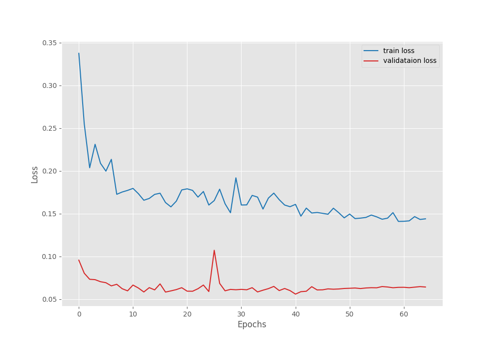
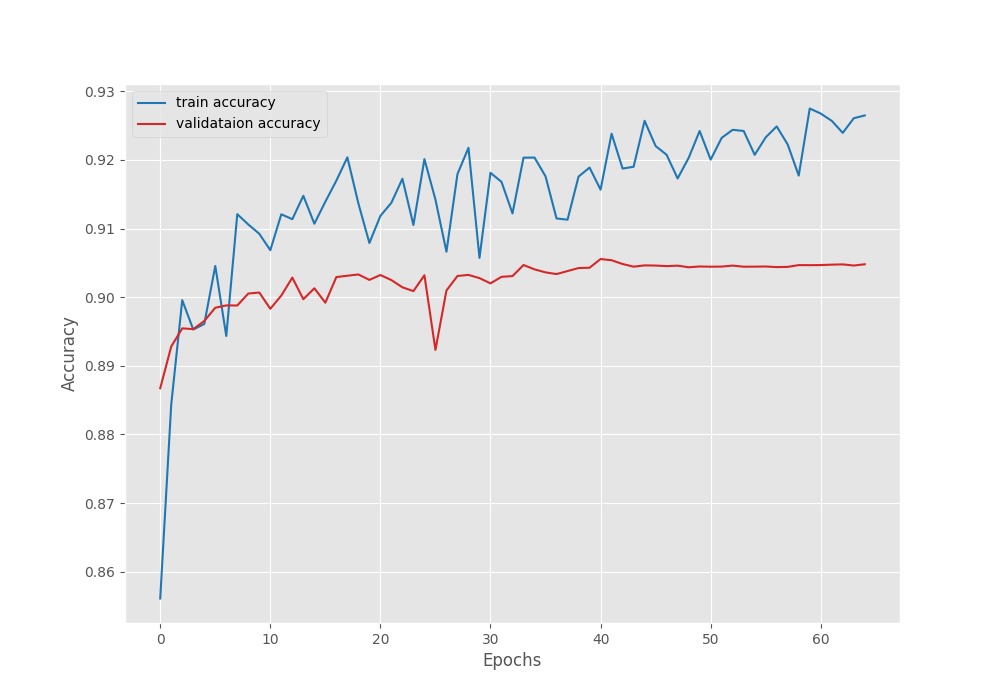
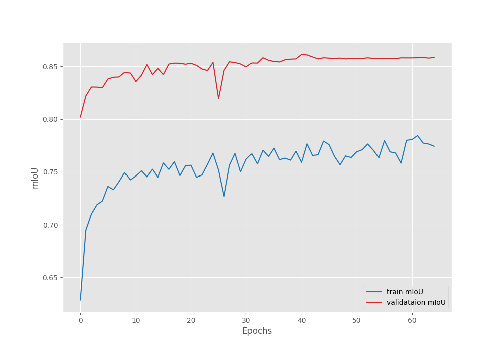
The plots seem to have plateaued after applying the learning rate scheduler. It may be worthwhile to train the model a bit longer than 45 epochs before applying the scheduler.
In the fine-tuning case, the model reached a mean IoU of more than 83% by the end of epoch 3 compared to 82% in the case of transfer learning.
Analysis and Takeaways
As we have completed the fine-tuning and transfer learning experiments for DINOv2 segmentation, we have a few interesting points to discuss.
- We gained a mean IoU of 2.4% when fine-tuning the model compared to transfer learning. Although we reached a higher metric, the computational requirement and training time were higher as we were training 22 million parameters compared to just 6000 parameters.
- We used a very small batch size of 2 for both experiments due to GPU memory constraints. In semantic segmentation, the model training usually benefits from a higher batch size. It will be extremely worthwhile to run both experiments again with a higher batch size (12 or higher) and compare the results again.
- It might also be beneficial to look at different augmentations and transformations in the dataset preparation phase that can lead to a higher mean IoU during transfer learning. That way, we may be able to train just a few thousand parameters of the segmentation head and still be able to reach the performance of fine-tuning.
- The final point is regarding the real-world scenario. Although we ran the experiments for fine-tuning and transfer learning for DINOv2 segmentation here, we did not carry out inference on real-world scenarios. Furthermore, we did not touch upon the point of model optimization for deployment as well. We will explore these in future articles.
Summary and Conclusion
In this article, we carried out fine-tuning and transfer learning experiments for semantic segmentation using a modified DINOv2 model. After the experiments, we analyzed the results and discussed some future experiments that will shed more light on the benefits of both approaches. I hope that this article was worth your time.
If you have any questions, thoughts, or suggestions, please leave them in the comment section. I will surely address them.
You can contact me using the Contact section. You can also find me on LinkedIn, and Twitter.

Great 👍
Thank you, Tilak.